Time-weighted averages and integrals

Time weighted averages and integrals are used in cases where a time series is not evenly sampled. Time series data points are often evenly spaced, for example every 30 seconds, or every hour. But sometimes data points are recorded irregularly, for example if a value has a large change, or changes quickly. Computing an average using data that is not evenly sampled is not always useful.

For example, if you have a lot of ice cream in freezers, you need to make sure the ice cream stays within a 0-10℉ (-20 to -12℃) temperature range. The temperature in the freezer can vary if folks are opening and closing the door, but the ice cream only has a problem if the temperature is out of range for a long time. You can set your sensors in the freezer to sample every five minutes while the temperature is in range, and every 30 seconds while the temperature is out of range. If the results are generally stable, but with some quick moving transients, an average of all the data points weights the transient values too highly. A time weighted average weights each value by the duration over which it occurred based on the points around it, producing much more accurate results.

Time weighted integrals are useful when you need a time-weighted sum of irregularly sampled data. For example, if you bill your users based on irregularly sampled CPU usage, you need to find the total area under the graph of their CPU usage. You can use a time-weighted integral to find the total CPU-hours used by a user over a given time period.

• For more information about how time-weighted averages work, read our [time-weighted averages blog][blog-timeweight].
• For more information about time-weighted average API calls, see the [hyperfunction API documentation][hyperfunctions-api-timeweight].

===== PAGE: https://docs.tigerdata.com/use-timescale/hyperfunctions/about-hyperfunctions/ =====

About TimescaleDB hyperfunctions

TimescaleDB hyperfunctions are a specialized set of functions that power real-time analytics on time series and events. IoT devices, IT systems, marketing analytics, user behavior, financial metrics, cryptocurrency - these are only a few examples of domains where hyperfunctions can make a huge difference. Hyperfunctions provide you with meaningful, actionable insights in real time.

Tiger Cloud includes all hyperfunctions by default, while self-hosted TimescaleDB includes a subset of them. For additional hyperfunctions, install the [TimescaleDB Toolkit][install-toolkit] Postgres extension.

Available hyperfunctions

Here is a list of all the hyperfunctions provided by TimescaleDB. Hyperfunctions with a tick in the Toolkit column require an installation of TimescaleDB Toolkit for self-hosted deployments. Hyperfunctions with a tick in the Experimental column are still under development.

Experimental features could have bugs. They might not be backwards compatible, and could be removed in future releases. Use these features at your own risk, and do not use any experimental features in production.

When you upgrade the timescaledb extension, the experimental schema is removed by default. To use experimental features after an upgrade, you need to add the experimental schema again.

<HyperfunctionTable includeExperimental />

For more information about each of the API calls listed in this table, see the [hyperfunction API documentation][api-hyperfunctions].

Function pipelines

Function pipelines are an experimental feature, designed to radically improve the developer ergonomics of analyzing data in Postgres and SQL, by applying principles from functional programming and popular tools like Python's Pandas, and PromQL.

SQL is the best language for data analysis, but it is not perfect, and at times can get quite unwieldy. For example, this query gets data from the last day from the measurements table, sorts the data by the time column, calculates the delta between the values, takes the absolute value of the delta, and then takes the sum of the result of the previous steps:

SELECT device id,
sum(abs_delta) as volatility
FROM (
 SELECT device_id,
abs(val - lag(val) OVER last_day) as abs_delta
FROM measurements
WHERE ts >= now()-'1 day'::interval) calc_delta
GROUP BY device_id;

You can express the same query with a function pipeline like this:

SELECT device_id,
 timevector(ts, val) -> sort() -> delta() -> abs() -> sum() as volatility
FROM measurements
WHERE ts >= now()-'1 day'::interval
GROUP BY device_id;

Function pipelines are completely SQL compliant, meaning that any tool that speaks SQL is able to support data analysis using function pipelines.

For more information about how function pipelines work, read our [blog post][blog-function-pipelines].

Toolkit feature development

TimescaleDB Toolkit features are developed in the open. As features are developed they are categorized as experimental, beta, stable, or deprecated. This documentation covers the stable features, but more information on our experimental features in development can be found in the [Toolkit repository][gh-docs].

Contribute to TimescaleDB Toolkit

We want and need your feedback! What are the frustrating parts of analyzing time-series data? What takes far more code than you feel it should? What runs slowly, or only runs quickly after many rewrites? We want to solve community-wide problems and incorporate as much feedback as possible.

• Join the [discussion][gh-discussions].
• Check out the [proposed features][gh-proposed].
• Explore the current [feature requests][gh-requests].
• Add your own [feature request][gh-newissue].

===== PAGE: https://docs.tigerdata.com/use-timescale/hyperfunctions/approx-count-distincts/ =====

Approximate count distincts

Approximate count distincts are typically used to find the number of unique values, or cardinality, in a large dataset. When you calculate cardinality in a dataset, the time it takes to process the query is proportional to how large the dataset is. So if you wanted to find the cardinality of a dataset that contained only 20 entries, the calculation would be very fast. Finding the cardinality of a dataset that contains 20 million entries, however, can take a significant amount of time and compute resources. Approximate count distincts do not calculate the exact cardinality of a dataset, but rather estimate the number of unique values, to reduce memory consumption and improve compute time by avoiding spilling the intermediate results to the secondary storage.

===== PAGE: https://docs.tigerdata.com/use-timescale/hyperfunctions/gapfilling-interpolation/ =====

Gapfilling and interpolation

Most time-series data analysis techniques aggregate data into fixed time intervals, which smooths the data and makes it easier to interpret and analyze. When you write queries for data in this form, you need an efficient way to aggregate raw observations, which are often noisy and irregular, in to fixed time intervals. TimescaleDB does this using time bucketing, which gives a clear picture of the important data trends using a concise, declarative SQL query.

Sorting data into time buckets works well in most cases, but problems can arise if there are gaps in the data. This can happen if you have irregular sampling intervals, or you have experienced an outage of some sort. You can use a gapfilling function to create additional rows of data in any gaps, ensuring that the returned rows are in chronological order, and contiguous.

• For more information about how gapfilling works, read our [gapfilling blog][blog-gapfilling].
• For more information about gapfilling and interpolation API calls, see the [hyperfunction API documentation][hyperfunctions-api-gapfilling].

===== PAGE: https://docs.tigerdata.com/use-timescale/hyperfunctions/approximate-percentile/ =====

Approximate percentiles

TimescaleDB uses approximation algorithms to calculate a percentile without requiring all of the data. This also makes them more compatible with continuous aggregates.

By default, TimescaleDB Toolkit uses uddsketch, but you can also choose to use tdigest. For more information about these algorithms, see the [advanced aggregation methods][advanced-agg] documentation.

Run an approximate percentage query

In this procedure, we use an example table called response_times that contains information about how long a server takes to respond to API calls.

Running an approximate percentage query

1. At the psql prompt, create a continuous aggregate that computes the daily aggregates:

   CREATE MATERIALIZED VIEW response_times_daily
   WITH (timescaledb.continuous)
   AS SELECT
     time_bucket('1 day'::interval, ts) as bucket,
     percentile_agg(response_time_ms)
   FROM response_times
   GROUP BY 1;

2. Re-aggregate the aggregate to get the last 30 days, and look for the ninety-fifth percentile:

   SELECT approx_percentile(0.95, percentile_agg) as threshold
   FROM response_times_daily
   WHERE bucket >= time_bucket('1 day'::interval, now() - '30 days'::interval);

3. You can also create an alert:

   WITH t as (SELECT approx_percentile(0.95, percentile_agg(percentile_agg)) as threshold
   FROM response_times_daily
   WHERE bucket >= time_bucket('1 day'::interval, now() - '30 days'::interval))
   
   SELECT count(*)
   FROM response_times
   WHERE ts > now()- '1 minute'::interval
   AND response_time_ms > (SELECT threshold FROM t);

For more information about percentile approximation API calls, see the [hyperfunction API documentation][hyperfunctions-api-approx-percentile].

===== PAGE: https://docs.tigerdata.com/use-timescale/hyperfunctions/index/ =====

Hyperfunctions

Real-time analytics demands more than basic SQL functions, efficient computation becomes essential as datasets grow in size and complexity. That’s where TimescaleDB hyperfunctions come in: high-performance, SQL-native functions purpose-built for time-series analysis. They are designed to process, aggregate, and analyze large volumes of data with maximum efficiency while maintaining consistently high performance. With hyperfunctions, you can run sophisticated analytical queries and extract meaningful insights in real time.

Hyperfunctions introduce partial aggregation, letting TimescaleDB store intermediate states instead of raw data or final results. These partials can be merged later for rollups (consolidation), eliminating costly reprocessing and slashing compute overhead, especially when paired with continuous aggregates.

Take tracking p95 latency across thousands of app instances as an example:

• With standard SQL, every rollup requires rescanning and resorting massive datasets.
• With TimescaleDB, the percentile_agg hyperfunction stores a compact state per minute, which you simply merge to get hourly or daily percentiles—no full reprocess needed.

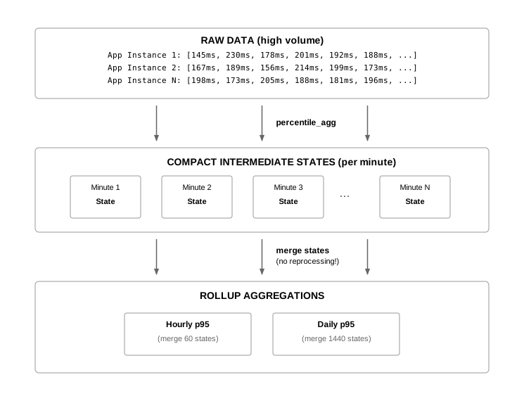
The result? Scalable, real-time percentile analytics that deliver fast, accurate insights across high-ingest, high-resolution data, while keeping resource use lean.

Tiger Cloud includes all hyperfunctions by default, while self-hosted TimescaleDB includes a subset of them. To include all hyperfunctions with TimescaleDB, install the [TimescaleDB Toolkit][install-toolkit] Postgres extension on your self-hosted Postgres deployment.

For more information, read the [hyperfunctions blog post][hyperfunctions-blog].

Learn hyperfunction basics and install TimescaleDB Toolkit

• [Learn about hyperfunctions][about-hyperfunctions] to understand how they work before using them.
• Install the [TimescaleDB Toolkit extension][install-toolkit] to access more hyperfunctions on self-hosted TimescaleDB.

Browse hyperfunctions and TimescaleDB Toolkit features by category

===== PAGE: https://docs.tigerdata.com/use-timescale/hyperfunctions/hyperloglog/ =====

Hyperloglog

Hyperloglog is typically used to find the cardinality of very large datasets. If you want to find the number of unique values, or cardinality, in a dataset, the time it takes to process this query is proportional to how large the dataset is. So if you wanted to find the cardinality of a dataset that contained only 20 entries, the calculation would be very fast. Finding the cardinality of a dataset that contains 20 million entries, however, can take a significant amount of time and compute resources.

Hyperloglog does not calculate the exact cardinality of a dataset, but rather estimates the number of unique values. It does this by converting the original data into a hash of random numbers that represents the cardinality of the dataset. This is not a perfect calculation of the cardinality, but it is usually within a margin of error of 2%.

The benefit of hyperloglog on time-series data is that it can continue to calculate the approximate cardinality of a dataset as it changes over time. It does this by adding an entry to the hyperloglog hash as new data is retrieved, rather than recalculating the result for the entire dataset every time it is needed. This makes it an ideal candidate for using with continuous aggregates.

For more information about approximate count distinct API calls, see the [hyperfunction API documentation][hyperfunctions-api-approx-count-distincts].

===== PAGE: https://docs.tigerdata.com/use-timescale/hyperfunctions/time-bucket-gapfill/ =====

Time bucket gapfill

Sometimes data sorted into time buckets can have gaps. This can happen if you have irregular sampling intervals, or you have experienced an outage of some sort. If you have a time bucket that has no data at all, the average returned from the time bucket is NULL, which could cause problems. You can use a gapfilling function to create additional rows of data in any gaps, ensuring that the returned rows are in chronological order, and contiguous. The time bucket gapfill function creates a contiguous set of time buckets but does not fill the rows with data. You can create data for the new rows using another function, such as last observation carried forward (LOCF), or interpolation.

For more information about gapfilling and interpolation API calls, see the [hyperfunction API documentation][hyperfunctions-api-gapfilling].

===== PAGE: https://docs.tigerdata.com/use-timescale/hyperfunctions/percentile-approx/ =====

Percentile approximation

In general, percentiles are useful for understanding the distribution of data. The fiftieth percentile is the point at which half of your data is greater and half is lesser. The tenth percentile is the point at which 90% of the data is greater, and 10% is lesser. The ninety-ninth percentile is the point at which 1% is greater, and 99% is lesser.

The fiftieth percentile, or median, is often a more useful measure than the average, especially when your data contains outliers. Outliers can dramatically change the average, but do not affect the median as much. For example, if you have three rooms in your house and two of them are 40℉ (4℃) and one is 130℉ (54℃), the average room temperature is 70℉ (21℃), which doesn't tell you much. However, the fiftieth percentile temperature is 40℉ (4℃), which tells you that at least half your rooms are at refrigerator temperatures (also, you should probably get your heating checked!)

Percentiles are sometimes avoided because calculating them requires more CPU and memory than an average or other aggregate measures. This is because an exact computation of the percentile needs the full dataset as an ordered list. TimescaleDB uses approximation algorithms to calculate a percentile without requiring all of the data. This also makes them more compatible with continuous aggregates. By default, TimescaleDB uses uddsketch, but you can also choose to use tdigest. For more information about these algorithms, see the [advanced aggregation methods][advanced-agg] documentation.

Technically, a percentile divides a group into 100 equally sized pieces, while a quantile divides a group into an arbitrary number of pieces. Because we don't always use exactly 100 buckets, "quantile" is the more technically correct term in this case. However, we use the word "percentile" because it's a more common word for this type of function.

• For more information about how percentile approximation works, read our [percentile approximation blog][blog-percentile-approx].
• For more information about percentile approximation API calls, see the [hyperfunction API documentation][hyperfunctions-api-approx-percentile].

===== PAGE: https://docs.tigerdata.com/use-timescale/hyperfunctions/advanced-agg/ =====

Percentile approximation advanced aggregation methods

TimescaleDB uses approximation algorithms to calculate a percentile without requiring all of the data. This also makes them more compatible with continuous aggregates. By default, TimescaleDB uses uddsketch, but you can also choose to use tdigest. This section describes the different methods, and helps you to decide which one you should use.

uddsketch is the default algorithm. It uses exponentially sized buckets to guarantee the approximation falls within a known error range, relative to the true discrete percentile. This algorithm offers the ability to tune the size and maximum error target of the sketch.

tdigest buckets data more aggressively toward the center of the quantile range, giving it greater accuracy at the tails of the range, around 0.001 or 0.995.

Choose the right algorithm

Each algorithm has different features, which can make one better than another depending on your use case. Here are some of the differences to consider when choosing an algorithm:

Before you begin, it is important to understand that the formal definition for a percentile is imprecise, and there are different methods for determining what the true percentile actually is. In Postgres, given a target percentile p, [percentile_disc][pg-percentile] returns the smallest element of a set, so that p percent of the set is less than that element. However, [percentile_cont][pg-percentile] returns an interpolated value between the two nearest matches for p. In practice, the difference between these methods is very small but, if it matters to your use case, keep in mind that tdigest approximates the continuous percentile, while uddsketch provides an estimate of the discrete value.

Think about the types of percentiles you're most interested in. tdigest is optimized for more accurate estimates at the extremes, and less accurate estimates near the median. If your workflow involves estimating ninety-ninth percentiles, then choose tdigest. If you're more concerned about getting highly accurate median estimates, choose uddsketch.

The algorithms differ in the way they estimate data. uddsketch has a stable bucketing function, so it always returns the same percentile estimate for the same underlying data, regardless of how it is ordered or re-aggregated. On the other hand, tdigest builds up incremental buckets based on the average of nearby points, which can result in some subtle differences in estimates based on the same data unless the order and batching of the aggregation is strictly controlled, which is sometimes difficult to do in Postgres. If stable estimates are important to you, choose uddsketch.

Calculating precise error bars for tdigest can be difficult, especially when merging multiple sub-digests into a larger one. This can occur through summary aggregation, or parallelization of the normal point aggregate. If you need to tightly characterize your errors, choose uddsketch. However, because uddsketch uses exponential bucketing to provide a guaranteed relative error, it can cause some wildly varying absolute errors if the dataset covers a large range. For example, if the data is evenly distributed over the range [1,100], estimates at the high end of the percentile range have about 100 times the absolute error of those at the low end of the range. This gets much more extreme if the data range is [0,100]. If having a stable absolute error is important to your use case, choose tdigest.

While both algorithms are likely to get smaller and faster with future optimizations, uddsketch generally requires a smaller memory footprint than tdigest, and a correspondingly smaller disk footprint for any continuous aggregates. Regardless of the algorithm you choose, the best way to improve the accuracy of your percentile estimates is to increase the number of buckets, which is simpler to do with uddsketch. If your use case does not get a clear benefit from using tdigest, the default uddsketch is your best choice.

For some more technical details and usage examples of the different algorithms, see the developer documentation for [uddsketch][gh-uddsketch] and [tdigest][gh-tdigest].

===== PAGE: https://docs.tigerdata.com/use-timescale/hyperfunctions/locf/ =====

Last observation carried forward

Last observation carried forward (LOCF) is a form of linear interpolation used to fill gaps in your data. It takes the last known value and uses it as a replacement for the missing data.

For more information about gapfilling and interpolation API calls, see the [hyperfunction API documentation][hyperfunctions-api-gapfilling].

===== PAGE: https://docs.tigerdata.com/use-timescale/hyperfunctions/stats-aggs/ =====

Statistical aggregation

To make common statistical aggregates easier to work with in window functions and continuous aggregates, TimescaleDB provides common statistical aggregates in a slightly different form than otherwise available in Postgres.

This example calculates the average, standard deviation, and kurtosis of a value in the measurements table:

SELECT
    time_bucket('10 min'::interval, ts),
    average(stats_agg(val)),
    stddev(stats_agg(val), 'pop'),
    kurtosis(stats_agg(val), 'pop')
FROM measurements
GROUP BY 1;

This uses a two-step aggregation process. The first step is an aggregation step (stats_agg(val)), which creates a machine-readable form of the aggregate. The second step is an accessor. The available accessors are average, stddev, and kurtosis. The accessors run final calculations and output the calculated value in a human-readable way. This makes it easier to construct your queries, because it distinguishes the parameters, and makes it clear which aggregates are being re-aggregated or rolled up. Additionally, because this query syntax is used in all TimescaleDB Toolkit queries, when you are used to it, you can use it to construct more and more complicated queries.

A more complex example uses window functions to calculate tumbling window statistical aggregates. The statistical aggregate is first calculated over each minute in the subquery and then the rolling aggregate is used to re-aggregate it over each 15 minute period preceding. The accessors remain the same as the previous example:

SELECT
    bucket,
    average(rolling(stats_agg) OVER fifteen_min),
    stddev(rolling(stats_agg) OVER fifteen_min, 'pop'),
    kurtosis(rolling(stats_agg) OVER fifteen_min, 'pop')
FROM (SELECT
        time_bucket('1 min'::interval, ts) AS bucket,
        stats_agg(val)
     FROM measurements
     GROUP BY 1) AS stats
WINDOW fifteen_min as (ORDER BY bucket ASC RANGE '15 minutes' PRECEDING);

For some more technical details and usage examples of the two-step aggregation method, see the [blog post on aggregates][blog-aggregates] or the [developer documentation][gh-two-step-agg].

The stats_agg aggregate is available in two forms, a one-dimensional aggregate shown earlier in this section, and a two-dimensional aggregate. The two-dimensional aggregate takes in two variables (Y, X), which are dependent and independent variables respectively. The two-dimensional aggregate performs all the same calculations on each individual variable as performing separate one-dimensional aggregates would, and additionally performs linear regression on the two variables. Accessors for one-dimensional values append a _y or _x to the name. For example:

SELECT
    average_y(stats_agg(val2, val1)), -- equivalent to average(stats_agg(val2))
    stddev_x(stats_agg(val2, val1)), -- equivalent to stddev(stats_agg(val1))
    slope(stats_agg(val2, val1)) -- the slope of the least squares fit line of the values in val2 & val1
FROM measurements_multival;

For more information about statistical aggregation API calls, see the [hyperfunction API documentation][hyperfunctions-api-stats-agg].

===== PAGE: https://docs.tigerdata.com/use-timescale/hyperfunctions/counter-aggregation/ =====

Counter aggregation

When you are monitoring application performance, there are two main types of metrics that you can collect: gauges, and counters. Gauges fluctuate up and down, like temperature or speed, while counters always increase, like the total number of miles travelled in a vehicle.

When you process counter data, it is usually assumed that if the value of the counter goes down, the counter has been reset. For example, if you wanted to count the total number of miles travelled in a vehicle, you would expect the values to continuously increase: 1, 2, 3, 4, and so on. If the counter reset to 0, you would expect that this was a new trip, or an entirely new vehicle. This can become a problem if you want to continue counting from where you left off, rather than resetting to 0. A reset could occur if you have had a short server outage, or any number of other reasons. To get around this, you can analyze counter data by looking at the change over time, which accounts for resets.

Accounting for resets can be difficult to do in SQL, so TimescaleDB has developed aggregate and accessor functions that handle calculations for counters in a more practical way.

Counter aggregates can be used in continuous aggregates, even though they are not parallelizable in Postgres. For more information, see the section on parallelism and ordering.

For more information about counter aggregation API calls, see the [hyperfunction API documentation][hyperfunctions-api-counter-agg].

Run a counter aggregate query using a delta function

In this procedure, we are using an example table called example that contains counter data.

Running a counter aggregate query using a delta function

1. Create a table called example:

   CREATE TABLE example (
       measure_id      BIGINT,
       ts              TIMESTAMPTZ ,
       val             DOUBLE PRECISION,
       PRIMARY KEY (measure_id, ts)
   );

2. Create a counter aggregate and the delta accessor function. This gives you the change in the counter's value over the time period, accounting for any resets. This allows you to search for fifteen minute periods where the counter increased by a larger or smaller amount:

   SELECT measure_id,
       delta(
           counter_agg(ts, val)
       )
   FROM example
   GROUP BY measure_id;

3. You can also use the time_bucket function to produce a series of deltas over fifteen minute increments:

   SELECT measure_id,
       time_bucket('15 min'::interval, ts) as bucket,
       delta(
           counter_agg(ts, val)
       )
   FROM example
   GROUP BY measure_id, time_bucket('15 min'::interval, ts);

Run a counter aggregate query using an extrapolated delta function

If your series is less regular, the deltas are affected by the number of samples in each fifteen minute period. You can improve this by using the extrapolated_delta function. To do this, you need to provide bounds that define where to extrapolate to. In this example, we use the time_bucket_range function, which works in the same way as time_bucket but produces an open ended range of all the times in the bucket. This example also uses a CTE to do the counter aggregation, which makes it a little easier to understand what's going on in each part.

Running a counter aggregate query using an extrapolated delta function

1. Create a hypertable called example:

   CREATE TABLE example (
       measure_id      BIGINT,
       ts              TIMESTAMPTZ ,
       val             DOUBLE PRECISION,
       PRIMARY KEY (measure_id, ts)
   ) WITH (
     tsdb.hypertable,
     tsdb.partition_column='ts',
     tsdb.chunk_interval='15 days'
   );

If you are self-hosting TimescaleDB v2.19.3 and below, create a [Postgres relational table][pg-create-table], then convert it using [create_hypertable][create_hypertable]. You then enable hypercore with a call to [ALTER TABLE][alter_table_hypercore].

1. Create a counter aggregate and the extrapolated delta function:

   with t as (
       SELECT measure_id,
           time_bucket('15 min'::interval, ts) as bucket,
           counter_agg(ts, val, toolkit_experimental.time_bucket_range('15 min'::interval, ts))
       FROM example
       GROUP BY measure_id, time_bucket('15 min'::interval, ts))
   SELECT time_bucket,
       extrapolated_delta(counter_agg, method => 'prometheus')
   FROM t ;

In this procedure, Prometheus is used to do the extrapolation. TimescaleDB's current extrapolation function is built to mimic the Prometheus project's increase function, which measures the change of a counter extrapolated to the edges of the queried region.

Run a counter aggregate query with a continuous aggregate

Your counter aggregate might be more useful if you make a continuous aggregate out of it.

1. Create the continuous aggregate:

   CREATE MATERIALIZED VIEW example_15
   WITH (timescaledb.continuous)
   AS SELECT measure_id,
       time_bucket('15 min'::interval, ts) as bucket,
       counter_agg(ts, val, time_bucket_range('15 min'::interval, ts))
   FROM example
   GROUP BY measure_id, time_bucket('15 min'::interval, ts);

2. You can also re-aggregate from the continuous aggregate into a larger bucket size:

   SELECT
       measure_id,
       time_bucket('1 day'::interval, bucket),
       delta(
           rollup(counter_agg)
       )
   FROM example_15
   GROUP BY measure_id, time_bucket('1 day'::interval, bucket);

Parallelism and ordering

The counter reset calculations require a strict ordering of inputs, which means they are not parallelizable in Postgres. This is because Postgres handles parallelism by issuing rows randomly to workers. However, if your parallelism can guarantee sets of rows that are disjointed in time, the algorithm can be parallelized, as long as it is within a time range, and all rows go to the same worker. This is the case for both continuous aggregates and for distributed hypertables, as long as the partitioning keys are in the group by, even though the aggregate itself doesn't really make sense otherwise.

For more information about parallelism and ordering, see our [developer documentation][gh-parallelism-ordering]

===== PAGE: https://docs.tigerdata.com/use-timescale/hyperfunctions/heartbeat-agg/ =====

Heartbeat aggregation

Given a series of timestamped health checks, it can be tricky to determine the overall health of a system over a given interval. Postgres provides window functions that you use to get a sense of where unhealthy gaps are, but they can be somewhat awkward to use efficiently.

This is one of the many cases where hyperfunctions provide an efficient, simple solution for a frequently occurring problem. Heartbeat aggregation helps analyze event-based time-series data with intermittent or irregular signals.

This example uses the [SustData public dataset][sustdata]. This dataset tracks the power usage of a small number of apartments and houses over four different deployment intervals. The data is collected in one-minute samples from each unit.

When you have loaded the data into hypertables, you can create a materialized view containing weekly heartbeat aggregates for each of the units:

CREATE MATERIALIZED VIEW weekly_heartbeat AS
  SELECT
    time_bucket('1 week', tmstp) as week,
    iid as unit,
    deploy,
    heartbeat_agg(tmstp, time_bucket('1w', tmstp), '1w', '2m')
  FROM power_samples
  GROUP BY 1,2,3;

The heartbeat aggregate takes four parameters: the timestamp column, the start of the interval, the length of the interval, and how long the aggregate is considered live after each timestamp. This example uses 2 minutes as the heartbeat lifetime to give some tolerance for small gaps.

You can use this data to see when you're receiving data for a particular unit. This example rolls up the weekly aggregates into a single aggregate, and then views the live ranges:

SELECT live_ranges(rollup(heartbeat_agg)) FROM weekly_heartbeat WHERE unit = 17;

                     live_ranges
-----------------------------------------------------
 ("2010-09-18 00:00:00+00","2011-03-27 01:01:50+00")
 ("2011-03-27 03:00:52+00","2011-07-03 00:01:00+00")
 ("2011-07-05 00:00:00+00","2011-08-21 00:01:00+00")
 ("2011-08-22 00:00:00+00","2011-08-25 00:01:00+00")
 ("2011-08-27 00:00:00+00","2011-09-06 00:01:00+00")
 ("2011-09-08 00:00:00+00","2011-09-29 00:01:00+00")
 ("2011-09-30 00:00:00+00","2011-10-04 00:01:00+00")
 ("2011-10-05 00:00:00+00","2011-10-17 00:01:00+00")
 ("2011-10-19 00:00:00+00","2011-11-09 00:01:00+00")
 ("2011-11-10 00:00:00+00","2011-11-14 00:01:00+00")
 ("2011-11-15 00:00:00+00","2011-11-18 00:01:00+00")
 ("2011-11-20 00:00:00+00","2011-11-23 00:01:00+00")
 ("2011-11-24 00:00:00+00","2011-12-01 00:01:00+00")
 ("2011-12-02 00:00:00+00","2011-12-12 00:01:00+00")
 ("2011-12-13 00:00:00+00","2012-01-12 00:01:00+00")
 ("2012-01-13 00:00:00+00","2012-02-03 00:01:00+00")
 ("2012-02-04 00:00:00+00","2012-02-10 00:01:00+00")
 ("2012-02-11 00:00:00+00","2012-03-25 01:01:50+00")
 ("2012-03-25 03:00:51+00","2012-04-11 00:01:00+00")

You can construct more elaborate queries. For example, to return the 5 units with the lowest uptime during the third deployment:

SELECT unit, uptime(rollup(heartbeat_agg))
FROM weekly_heartbeat
WHERE deploy = 3
GROUP BY unit
ORDER BY uptime LIMIT 5;

 unit |      uptime
------+-------------------
   31 | 203 days 22:05:00
   34 | 222 days 22:05:00
   32 | 222 days 22:05:00
   35 | 222 days 22:05:00
   30 | 222 days 22:05:00

Combine aggregates from different units to get the combined coverage. This example queries the interval where any part of a deployment was active:

SELECT deploy, live_ranges(rollup(heartbeat_agg))
FROM weekly_heartbeat group by deploy order by deploy;

 deploy |                     live_ranges
--------+-----------------------------------------------------
      1 | ("2010-07-29 00:00:00+00","2010-11-26 00:01:00+00")
      2 | ("2010-11-25 00:00:00+00","2011-03-27 01:01:59+00")
      2 | ("2011-03-27 03:00:00+00","2012-03-25 01:01:59+00")
      2 | ("2012-03-25 03:00:26+00","2012-04-17 00:01:00+00")
      2 | ("2012-04-20 00:00:00+00","2012-04-21 00:01:00+00")
      2 | ("2012-05-11 00:00:00+00","2012-05-13 00:01:00+00")
      2 | ("2013-02-20 00:00:00+00","2013-02-21 00:01:00+00")
      3 | ("2012-08-01 00:00:01+00","2013-03-31 01:01:16+00")
      3 | ("2013-03-31 03:00:03+00","2013-05-22 00:01:00+00")
      4 | ("2013-07-31 00:00:00+00","2014-03-30 01:01:49+00")
      4 | ("2014-03-30 03:00:01+00","2014-04-25 00:01:00+00")

Then use this data to make observations and draw conclusions:

• The second deployment had a lot more problems than the other ones.
• There were some readings from February 2013 that were incorrectly categorized as a second deployment.
• The timestamps are given in a local time without time zone, resulting in some missing hours around springtime daylight savings time changes.

For more information about heartbeat aggregation API calls, see the [hyperfunction API documentation][hyperfunctions-api-heartbeat-agg].

===== PAGE: https://docs.tigerdata.com/use-timescale/hyperfunctions/troubleshoot-hyperfunctions/ =====

Troubleshooting hyperfunctions and TimescaleDB Toolkit

This section contains some ideas for troubleshooting common problems experienced with hyperfunctions and Toolkit.

Updating the Toolkit extension fails with an error saying no update path

In some cases, when you create the extension, or use the ALTER EXTENSION timescaledb_toolkit UPDATE command to update the Toolkit extension, it might fail with an error like this:

ERROR:  extension "timescaledb_toolkit" has no update path from version "1.2" to version "1.3"

This occurs if the list of available extensions does not include the version you are trying to upgrade to, and it can occur if the package was not installed correctly in the first place. To correct the problem, install the upgrade package, restart Postgres, verify the version, and then attempt the update again.