Query the Bitcoin blockchain

The financial industry is extremely data-heavy and relies on real-time and historical data for decision-making, risk assessment, fraud detection, and market analysis. Tiger Data simplifies management of these large volumes of data, while also providing you with meaningful analytical insights and optimizing storage costs.

In this tutorial, you use Tiger Cloud to ingest, store, and analyze transactions on the Bitcoin blockchain.

[Blockchains][blockchain-def] are, at their essence, a distributed database. The [transactions][transactions-def] in a blockchain are an example of time-series data. You can use TimescaleDB to query transactions on a blockchain, in exactly the same way as you might query time-series transactions in any other database.

Steps in this tutorial

This tutorial covers:

1. [Ingest data into a service][blockchain-dataset]: set up and connect to a Tiger Cloud service, create tables and hypertables, and ingest data.
2. [Query your data][blockchain-query]: obtain information, including finding the most recent transactions on the blockchain, and gathering information about the transactions using aggregation functions.
3. [Compress your data using hypercore][blockchain-compress]: compress data that is no longer needed for highest performance queries, but is still accessed regularly for real-time analytics.

When you've completed this tutorial, you can use the same dataset to [Analyze the Bitcoin data][analyze-blockchain], using TimescaleDB hyperfunctions.

===== PAGE: https://docs.tigerdata.com/tutorials/blockchain-analyze/ =====

Analyze the Bitcoin blockchain

The financial industry is extremely data-heavy and relies on real-time and historical data for decision-making, risk assessment, fraud detection, and market analysis. Tiger Data simplifies management of these large volumes of data, while also providing you with meaningful analytical insights and optimizing storage costs.

In this tutorial, you use Tiger Cloud to ingest, store, and analyze transactions on the Bitcoin blockchain.

[Blockchains][blockchain-def] are, at their essence, a distributed database. The [transactions][transactions-def] in a blockchain are an example of time-series data. You can use TimescaleDB to query transactions on a blockchain, in exactly the same way as you might query time-series transactions in any other database.

Prerequisites

Before you begin, make sure you have:

• Signed up for a [free Tiger Data account][cloud-install].
• Signed up for a [Grafana account][grafana-setup] to graph your queries.

Steps in this tutorial

This tutorial covers:

1. [Setting up your dataset][blockchain-dataset]
2. [Querying your dataset][blockchain-analyze]

About analyzing the Bitcoin blockchain with Tiger Cloud

This tutorial uses a sample Bitcoin dataset to show you how to aggregate blockchain transaction data, and construct queries to analyze information from the aggregations. The queries in this tutorial help you determine if a cryptocurrency has a high transaction fee, shows any correlation between transaction volumes and fees, or if it's expensive to mine.

It starts by setting up and connecting to a Tiger Cloud service, create tables, and load data into the tables using psql. If you have already completed the [beginner blockchain tutorial][blockchain-query], then you already have the dataset loaded, and you can skip straight to the queries.

You then learn how to conduct analysis on your dataset using Timescale hyperfunctions. It walks you through creating a series of continuous aggregates, and querying the aggregates to analyze the data. You can also use those queries to graph the output in Grafana.

===== PAGE: https://docs.tigerdata.com/tutorials/financial-tick-data/ =====

Analyze financial tick data with TimescaleDB

The financial industry is extremely data-heavy and relies on real-time and historical data for decision-making, risk assessment, fraud detection, and market analysis. Tiger Data simplifies management of these large volumes of data, while also providing you with meaningful analytical insights and optimizing storage costs.

To analyze financial data, you can chart the open, high, low, close, and volume (OHLCV) information for a financial asset. Using this data, you can create candlestick charts that make it easier to analyze the price changes of financial assets over time. You can use candlestick charts to examine trends in stock, cryptocurrency, or NFT prices.

In this tutorial, you use real raw financial data provided by [Twelve Data][twelve-data], create an aggregated candlestick view, query the aggregated data, and visualize the data in Grafana.

OHLCV data and candlestick charts

The financial sector regularly uses [candlestick charts][charts] to visualize the price change of an asset. Each candlestick represents a time period, such as one minute or one hour, and shows how the asset's price changed during that time.

Candlestick charts are generated from the open, high, low, close, and volume data for each financial asset during the time period. This is often abbreviated as OHLCV:

• Open: opening price
• High: highest price
• Low: lowest price
• Close: closing price
• Volume: volume of transactions

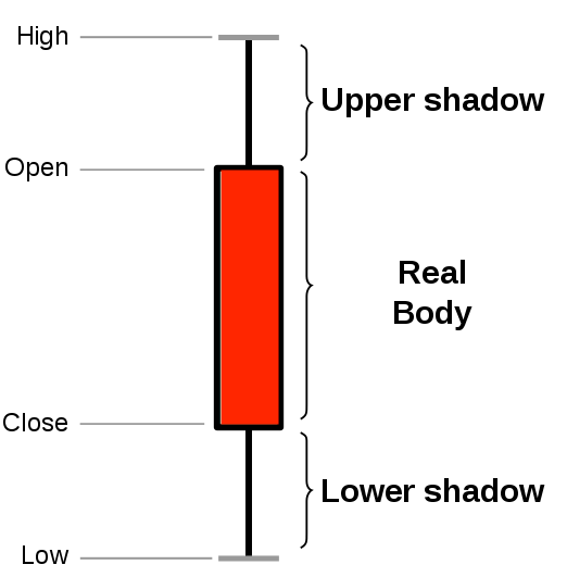
TimescaleDB is well suited to storing and analyzing financial candlestick data, and many Tiger Data community members use it for exactly this purpose. Check out these stories from some Tiger Datacommunity members:

• [How Trading Strategy built a data stack for crypto quant trading][trading-strategy]
• [How Messari uses data to open the cryptoeconomy to everyone][messari]
• [How I power a (successful) crypto trading bot with TimescaleDB][bot]

Steps in this tutorial

This tutorial shows you how to ingest real-time time-series data into a Tiger Cloud service:

1. [Ingest data into a service][financial-tick-dataset]: load data from [Twelve Data][twelve-data] into your TimescaleDB database.
2. [Query your dataset][financial-tick-query]: create candlestick views, query the aggregated data, and visualize the data in Grafana.
3. [Compress your data using hypercore][financial-tick-compress]: learn how to store and query your financial tick data more efficiently using compression feature of TimescaleDB.

To create candlestick views, query the aggregated data, and visualize the data in Grafana, see the [ingest real-time websocket data section][advanced-websocket].

===== PAGE: https://docs.tigerdata.com/tutorials/financial-ingest-real-time/ =====

Ingest real-time financial data using WebSocket

The financial industry is extremely data-heavy and relies on real-time and historical data for decision-making, risk assessment, fraud detection, and market analysis. Tiger Data simplifies management of these large volumes of data, while also providing you with meaningful analytical insights and optimizing storage costs.

This tutorial shows you how to ingest real-time time-series data into TimescaleDB using a websocket connection. The tutorial sets up a data pipeline to ingest real-time data from our data partner, [Twelve Data][twelve-data]. Twelve Data provides a number of different financial APIs, including stock, cryptocurrencies, foreign exchanges, and ETFs. It also supports websocket connections in case you want to update your database frequently. With websockets, you need to connect to the server, subscribe to symbols, and you can start receiving data in real-time during market hours.

When you complete this tutorial, you'll have a data pipeline set up that ingests real-time financial data into your Tiger Cloud.

This tutorial uses Python and the API [wrapper library][twelve-wrapper] provided by Twelve Data.

Prerequisites

Before you begin, make sure you have:

• Signed up for a [free Tiger Data account][cloud-install].
• Installed Python 3
• Signed up for [Twelve Data][twelve-signup]. The free tier is perfect for this tutorial.
• Made a note of your Twelve Data API key.

Steps in this tutorial

This tutorial covers:

1. [Setting up your dataset][financial-ingest-dataset]: Load data from [Twelve Data][twelve-data] into your TimescaleDB database.

2. [Querying your dataset][financial-ingest-query]: Create candlestick views, query the aggregated data, and visualize the data in Grafana.

   This tutorial shows you how to ingest real-time time-series data into a Tiger Cloud service using a websocket connection. To create candlestick views, query the aggregated data, and visualize the data in Grafana.

About OHLCV data and candlestick charts

The financial sector regularly uses [candlestick charts][charts] to visualize the price change of an asset. Each candlestick represents a time period, such as one minute or one hour, and shows how the asset's price changed during that time.

Candlestick charts are generated from the open, high, low, close, and volume data for each financial asset during the time period. This is often abbreviated as OHLCV:

• Open: opening price
• High: highest price
• Low: lowest price
• Close: closing price
• Volume: volume of transactions

TimescaleDB is well suited to storing and analyzing financial candlestick data, and many Tiger Datacommunity members use it for exactly this purpose.

===== PAGE: https://docs.tigerdata.com/api/hypertable/ =====

Hypertables and chunks

Tiger Cloud supercharges your real-time analytics by letting you run complex queries continuously, with near-zero latency. Under the hood, this is achieved by using hypertables—Postgres tables that automatically partition your time-series data by time and optionally by other dimensions. When you run a query, Tiger Cloud identifies the correct partition, called chunk, and runs the query on it, instead of going through the entire table.

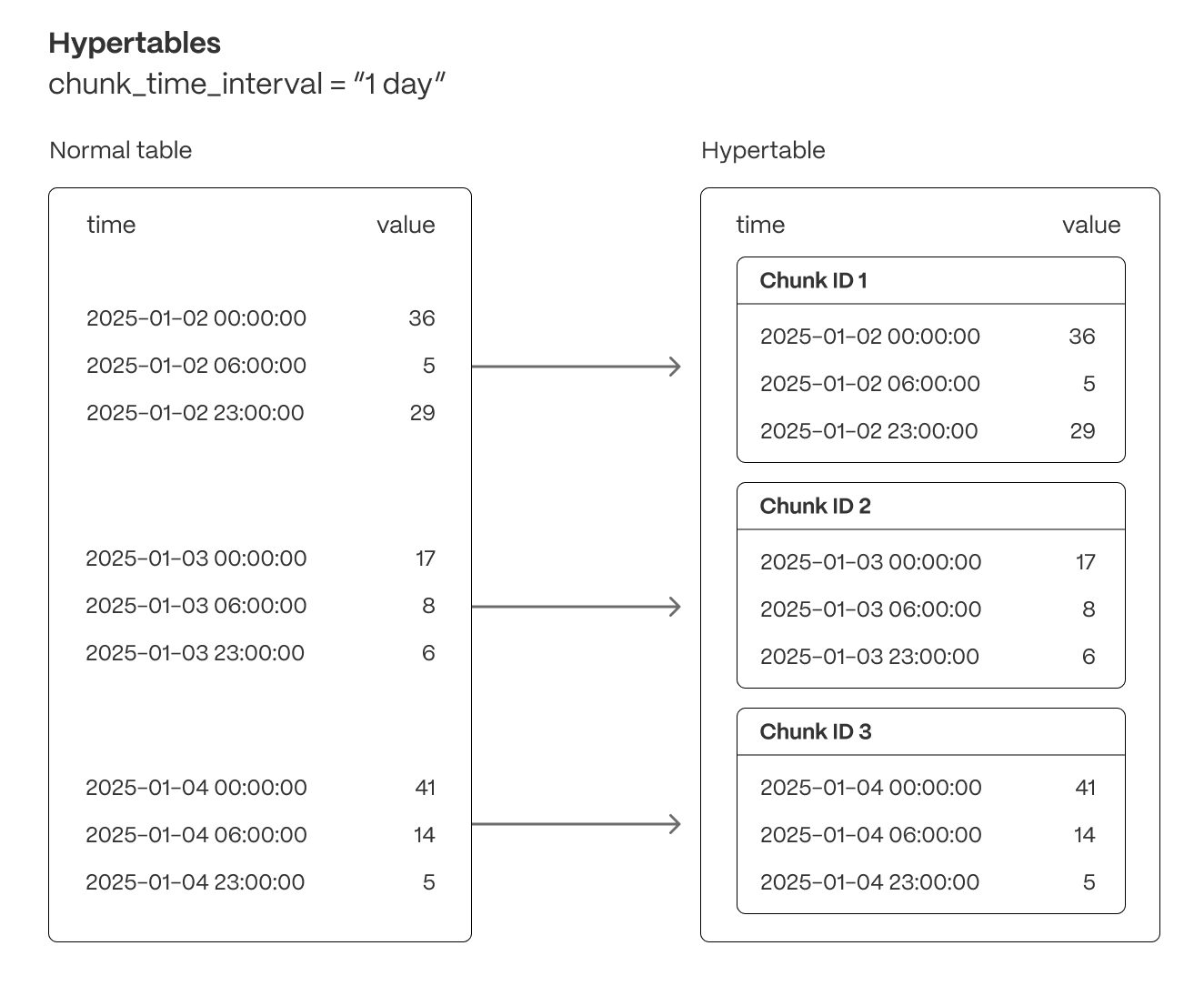
Hypertables offer the following benefits:

• Efficient data management with [automated partitioning by time][chunk-size]: Tiger Cloud splits your data into chunks that hold data from a specific time range. For example, one day or one week. You can configure this range to better suit your needs.

• Better performance with [strategic indexing][hypertable-indexes]: an index on time in the descending order is automatically created when you create a hypertable. More indexes are created on the chunk level, to optimize performance. You can create additional indexes, including unique indexes, on the columns you need.

• Faster queries with [chunk skipping][chunk-skipping]: Tiger Cloud skips the chunks that are irrelevant in the context of your query, dramatically reducing the time and resources needed to fetch results. Even more—you can enable chunk skipping on non-partitioning columns.

• Advanced data analysis with [hyperfunctions][hyperfunctions]: Tiger Cloud enables you to efficiently process, aggregate, and analyze significant volumes of data while maintaining high performance.

To top it all, there is no added complexity—you interact with hypertables in the same way as you would with regular Postgres tables. All the optimization magic happens behind the scenes.

Inheritance is not supported for hypertables and may lead to unexpected behavior.

For more information about using hypertables, including chunk size partitioning, see the [hypertable section][hypertable-docs].

The hypertable workflow

Best practice for using a hypertable is to:

1. Create a hypertable

   Create a [hypertable][hypertables-section] for your time-series data using [CREATE TABLE][hypertable-create-table]. For [efficient queries][secondary-indexes] on data in the columnstore, remember to segmentby the column you will use most often to filter your data. For example:

   CREATE TABLE conditions (
      time        TIMESTAMPTZ       NOT NULL,
      location    TEXT              NOT NULL,
      device      TEXT              NOT NULL,
      temperature DOUBLE PRECISION  NULL,
      humidity    DOUBLE PRECISION  NULL
   ) WITH (
      tsdb.hypertable,
      tsdb.partition_column='time',
      tsdb.segmentby = 'device',
      tsdb.orderby = 'time DESC'
   );

   If you are self-hosting TimescaleDB v2.19.3 and below, create a [Postgres relational table][pg-create-table], then convert it using [create_hypertable][create_hypertable]. You then enable hypercore with a call to [ALTER TABLE][alter_table_hypercore].

2. Set the columnstore policy

   CALL add_columnstore_policy('conditions', after => INTERVAL '1d');

===== PAGE: https://docs.tigerdata.com/api/hypercore/ =====

Hypercore

Hypercore is a hybrid row-columnar storage engine in TimescaleDB. It is designed specifically for real-time analytics and powered by time-series data. The advantage of hypercore is its ability to seamlessly switch between row-oriented and column-oriented storage, delivering the best of both worlds:

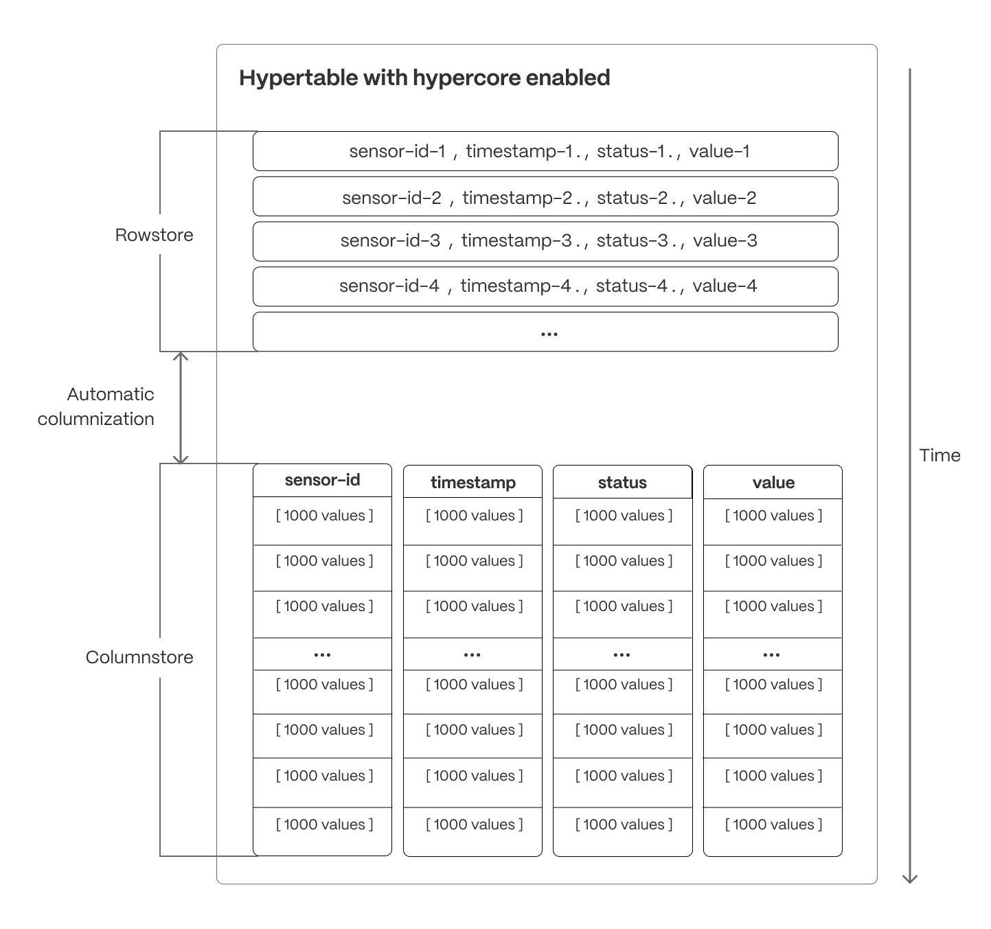
Hypercore solves the key challenges in real-time analytics:

• High ingest throughput
• Low-latency ingestion
• Fast query performance
• Efficient handling of data updates and late-arriving data
• Streamlined data management

Hypercore’s hybrid approach combines the benefits of row-oriented and column-oriented formats:

• Fast ingest with rowstore: new data is initially written to the rowstore, which is optimized for high-speed inserts and updates. This process ensures that real-time applications easily handle rapid streams of incoming data. Mutability—upserts, updates, and deletes happen seamlessly.

• Efficient analytics with columnstore: as the data cools and becomes more suited for analytics, it is automatically converted to the columnstore. This columnar format enables fast scanning and aggregation, optimizing performance for analytical workloads while also saving significant storage space.

• Faster queries on compressed data in columnstore: in the columnstore conversion, hypertable chunks are compressed by up to 98%, and organized for efficient, large-scale queries. Combined with [chunk skipping][chunk-skipping], this helps you save on storage costs and keeps your queries operating at lightning speed.

• Fast modification of compressed data in columnstore: just use SQL to add or modify data in the columnstore. TimescaleDB is optimized for superfast INSERT and UPSERT performance.

• Full mutability with transactional semantics: regardless of where data is stored, hypercore provides full ACID support. Like in a vanilla Postgres database, inserts and updates to the rowstore and columnstore are always consistent, and available to queries as soon as they are completed.

For an in-depth explanation of how hypertables and hypercore work, see the [Data model][data-model].

Since TimescaleDB v2.18.0

Hypercore workflow

Best practice for using hypercore is to:

1. Enable columnstore

   Create a [hypertable][hypertables-section] for your time-series data using [CREATE TABLE][hypertable-create-table]. For [efficient queries][secondary-indexes] on data in the columnstore, remember to segmentby the column you will use most often to filter your data. For example:

   • [Use CREATE TABLE for a hypertable][hypertable-create-table]

     CREATE TABLE crypto_ticks (
        "time" TIMESTAMPTZ,
        symbol TEXT,
        price DOUBLE PRECISION,
        day_volume NUMERIC
     ) WITH (
       tsdb.hypertable,
       tsdb.partition_column='time',
       tsdb.segmentby='symbol',
       tsdb.orderby='time DESC'
     );

     If you are self-hosting TimescaleDB v2.19.3 and below, create a [Postgres relational table][pg-create-table], then convert it using [create_hypertable][create_hypertable]. You then enable hypercore with a call to [ALTER TABLE][alter_table_hypercore].

   • [Use ALTER MATERIALIZED VIEW for a continuous aggregate][compression_continuous-aggregate]

     ALTER MATERIALIZED VIEW assets_candlestick_daily set (
        timescaledb.enable_columnstore = true,
        timescaledb.segmentby = 'symbol' );

2. Add a policy to move chunks to the columnstore at a specific time interval

   For example, 7 days after the data was added to the table:

   CALL add_columnstore_policy('crypto_ticks', after => INTERVAL '7d');

   See [add_columnstore_policy][add_columnstore_policy].

3. View the policies that you set or the policies that already exist

   SELECT * FROM timescaledb_information.jobs
   WHERE proc_name='policy_compression';

   See [timescaledb_information.jobs][informational-views].

You can also [convert_to_columnstore][convert_to_columnstore] and [convert_to_rowstore][convert_to_rowstore] manually for more fine-grained control over your data.

Limitations

Chunks in the columnstore have the following limitations:

• ROW LEVEL SECURITY is not supported on chunks in the columnstore.

===== PAGE: https://docs.tigerdata.com/api/continuous-aggregates/ =====

Continuous aggregates

In modern applications, data usually grows very quickly. This means that aggregating it into useful summaries can become very slow. If you are collecting data very frequently, you might want to aggregate your data into minutes or hours instead. For example, if an IoT device takes temperature readings every second, you might want to find the average temperature for each hour. Every time you run this query, the database needs to scan the entire table and recalculate the average. TimescaleDB makes aggregating data lightning fast, accurate, and easy with continuous aggregates.

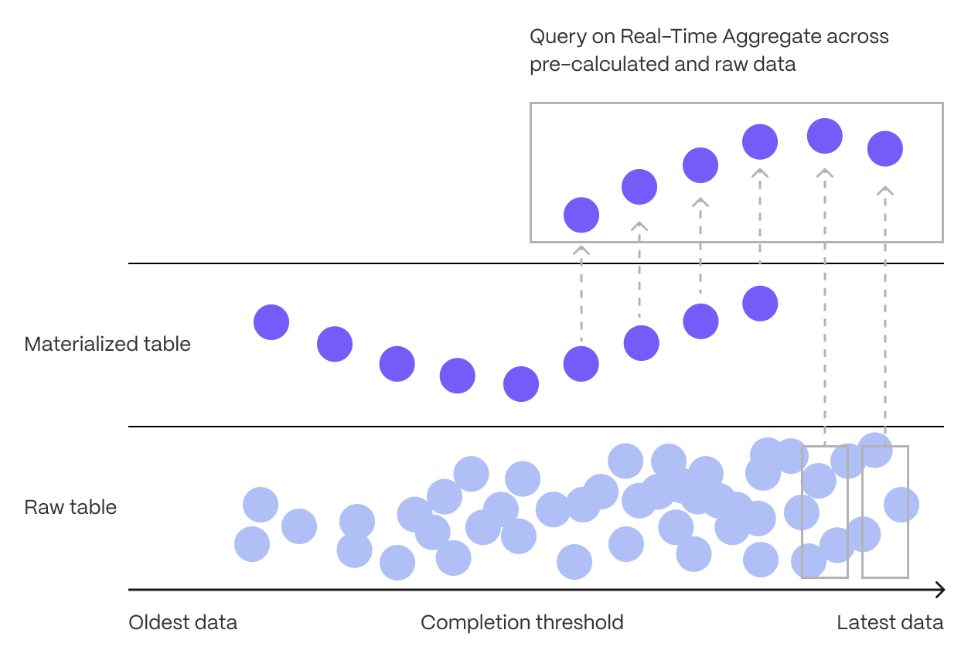
Continuous aggregates in TimescaleDB are a kind of hypertable that is refreshed automatically in the background as new data is added, or old data is modified. Changes to your dataset are tracked, and the hypertable behind the continuous aggregate is automatically updated in the background.

Continuous aggregates have a much lower maintenance burden than regular Postgres materialized views, because the whole view is not created from scratch on each refresh. This means that you can get on with working your data instead of maintaining your database.

Because continuous aggregates are based on hypertables, you can query them in exactly the same way as your other tables. This includes continuous aggregates in the rowstore, compressed into the [columnstore][hypercore], or [tiered to object storage][data-tiering]. You can even create [continuous aggregates on top of your continuous aggregates][hierarchical-caggs], for an even more fine-tuned aggregation.

[Real-time aggregation][real-time-aggregation] enables you to combine pre-aggregated data from the materialized view with the most recent raw data. This gives you up-to-date results on every query. In TimescaleDB v2.13 and later, real-time aggregates are DISABLED by default. In earlier versions, real-time aggregates are ENABLED by default; when you create a continuous aggregate, queries to that view include the results from the most recent raw data.

For more information about using continuous aggregates, see the documentation in [Use Tiger Data products][cagg-docs].

===== PAGE: https://docs.tigerdata.com/api/data-retention/ =====

Data retention

An intrinsic part of time-series data is that new data is accumulated and old data is rarely, if ever, updated. This means that the relevance of the data diminishes over time. It is therefore often desirable to delete old data to save disk space.

With TimescaleDB, you can manually remove old chunks of data or implement policies using these APIs.

For more information about creating a data retention policy, see the [data retention section][data-retention-howto].

===== PAGE: https://docs.tigerdata.com/api/jobs-automation/ =====

Jobs

Jobs allow you to run functions and procedures implemented in a language of your choice on a schedule within Timescale. This allows automatic periodic tasks that are not covered by existing policies and even enhancing existing policies with additional functionality.

The following APIs and views allow you to manage the jobs that you create and get details around automatic jobs used by other TimescaleDB functions like continuous aggregation refresh policies and data retention policies. To view the policies that you set or the policies that already exist, see [informational views][informational-views].

===== PAGE: https://docs.tigerdata.com/api/uuid-functions/ =====

UUIDv7 functions

UUIDv7 is a time-ordered UUID that includes a Unix timestamp (with millisecond precision) in its first 48 bits. Like other UUIDs, it uses 6 bits for version and variant info, and the remaining 74 bits are random.

UUIDv7 is ideal anywhere you create lots of records over time, not only observability. Advantages are:

• No extra column required to partition by time with sortability: you can sort UUIDv7 instances by their value. This is useful for ordering records by creation time without the need for a separate timestamp column.
• Indexing performance: UUIDv7s increase with time, so new rows append near the end of a B-tree instead of This results in fewer page splits, less fragmentation, faster inserts, and efficient time-range scans.
• Easy keyset pagination: WHERE id > :cursor and natural sharding.
• UUID: safe across services, replicas, and unique across distributed systems.

UUIDv7 also increases query speed by reducing the number of chunks scanned during queries. For example, in a database with 25 million rows, the following query runs in 25 seconds:

WITH ref AS (SELECT now() AS t0)
SELECT count(*) AS cnt_ts_filter
FROM events e, ref
WHERE uuid_timestamp(e.event_id) >= ref.t0 - INTERVAL '2 days';

Using UUIDv7 excludes chunks at startup and reduces the query time to 550ms:

WITH ref AS (SELECT now() AS t0)
SELECT count(*) AS cnt_boundary_filter
FROM events e, ref
WHERE e.event_id >= to_uuidv7_boundary(ref.t0 - INTERVAL '2 days')

You use UUIDvs for events, orders, messages, uploads, runs, jobs, spans, and more.

Examples

• High-rate event logs for observability and metrics:

  UUIDv7 gives you globally unique IDs (for traceability) and time windows (“last hour”), without the need for a separate created_at column. UUIDv7 create less churn because inserts land at the end of the index, and you can filter by time using UUIDv7 objects.

  • Last hour:

    SELECT count(*) FROM logs WHERE id >= to_uuidv7_boundary(now() - interval '1 hour');

  • Keyset pagination

    SELECT * FROM logs WHERE id > to_uuidv7($last_seen'::timestamptz, true) ORDER BY id LIMIT 1000;

• Workflow / durable execution runs:

  Each run needs a stable ID for joins and retries, and you often ask “what started since X?”. UUIDs help by serving both as the primary key and a time cursor across services. For example:

  SELECT run_id, status
  FROM runs
  WHERE run_id >= to_uuidv7_boundary(now() - interval '5 minutes')

• Orders / activity feeds / messages (SaaS apps):

  Human-readable timestamps are not mandatory in a table. However, you still need time-ordered pages and day/week ranges. UUIDv7 enables clean date windows and cursor pagination with just the ID. For example:

  SELECT * FROM orders
  WHERE id >= to_uuidv7('2025-08-01'::timestamptz, true)
  AND id <  to_uuidv7('2025-08-02'::timestamptz, true)
  ORDER BY id;

Functions

• [generate_uuidv7()][generate_uuidv7]: generate a version 7 UUID based on current time
• [to_uuidv7()][to_uuidv7]: create a version 7 UUID from a PostgreSQL timestamp
• [to_uuidv7_boundary()][to_uuidv7_boundary]: create a version 7 "boundary" UUID from a PostgreSQL timestamp
• [uuid_timestamp()][uuid_timestamp]: extract a PostgreSQL timestamp from a version 7 UUID
• [uuid_timestamp_micros()][uuid_timestamp_micros]: extract a PostgreSQL timestamp with microsecond precision from a version 7 UUID
• [uuid_version()][uuid_version]: extract the version of a UUID

===== PAGE: https://docs.tigerdata.com/api/approximate_row_count/ =====

approximate_row_count()

Get approximate row count for hypertable, distributed hypertable, or regular Postgres table based on catalog estimates. This function supports tables with nested inheritance and declarative partitioning.

The accuracy of approximate_row_count depends on the database having up-to-date statistics about the table or hypertable, which are updated by VACUUM, ANALYZE, and a few DDL commands. If you have auto-vacuum configured on your table or hypertable, or changes to the table are relatively infrequent, you might not need to explicitly ANALYZE your table as shown below. Otherwise, if your table statistics are too out-of-date, running this command updates your statistics and yields more accurate approximation results.

Samples

Get the approximate row count for a single hypertable.

ANALYZE conditions;

SELECT * FROM approximate_row_count('conditions');

The expected output:

approximate_row_count
----------------------
               240000

Required arguments

Name	Type	Description
relation	REGCLASS	Hypertable or regular Postgres table to get row count for.

===== PAGE: https://docs.tigerdata.com/api/first/ =====

first()

The first aggregate allows you to get the value of one column as ordered by another. For example, first(temperature, time) returns the earliest temperature value based on time within an aggregate group.

The last and first commands do not use indexes, they perform a sequential scan through the group. They are primarily used for ordered selection within a GROUP BY aggregate, and not as an alternative to an ORDER BY time DESC LIMIT 1 clause to find the latest value, which uses indexes.

Samples

Get the earliest temperature by device_id:

SELECT device_id, first(temp, time)
FROM metrics
GROUP BY device_id;

This example uses first and last with an aggregate filter, and avoids null values in the output:

SELECT
   TIME_BUCKET('5 MIN', time_column) AS interv,
   AVG(temperature) as avg_temp,
   first(temperature,time_column) FILTER(WHERE time_column IS NOT NULL) AS beg_temp,
   last(temperature,time_column) FILTER(WHERE time_column IS NOT NULL) AS end_temp
FROM sensors
GROUP BY interv

Required arguments

Name	Type	Description
value	TEXT	The value to return
time	TIMESTAMP or INTEGER	The timestamp to use for comparison

===== PAGE: https://docs.tigerdata.com/api/last/ =====

last()

The last aggregate allows you to get the value of one column as ordered by another. For example, last(temperature, time) returns the latest temperature value based on time within an aggregate group.

The last and first commands do not use indexes, they perform a sequential scan through the group. They are primarily used for ordered selection within a GROUP BY aggregate, and not as an alternative to an ORDER BY time DESC LIMIT 1 clause to find the latest value, which uses indexes.

Samples

Get the temperature every 5 minutes for each device over the past day:

SELECT device_id, time_bucket('5 minutes', time) AS interval,
  last(temp, time)
FROM metrics
WHERE time > now () - INTERVAL '1 day'
GROUP BY device_id, interval
ORDER BY interval DESC;

This example uses first and last with an aggregate filter, and avoids null values in the output:

SELECT
   TIME_BUCKET('5 MIN', time_column) AS interv,
   AVG(temperature) as avg_temp,
   first(temperature,time_column) FILTER(WHERE time_column IS NOT NULL) AS beg_temp,
   last(temperature,time_column) FILTER(WHERE time_column IS NOT NULL) AS end_temp
FROM sensors
GROUP BY interv

Required arguments

Name	Type	Description
value	ANY ELEMENT	The value to return
time	TIMESTAMP or INTEGER	The timestamp to use for comparison

===== PAGE: https://docs.tigerdata.com/api/histogram/ =====

histogram()

The histogram() function represents the distribution of a set of values as an array of equal-width buckets. It partitions the dataset into a specified number of buckets (nbuckets) ranging from the inputted min and max values.

The return value is an array containing nbuckets+2 buckets, with the middle nbuckets bins for values in the stated range, the first bucket at the head of the array for values under the lower min bound, and the last bucket for values greater than or equal to the max bound. Each bucket is inclusive on its lower bound, and exclusive on its upper bound. Therefore, values equal to the min are included in the bucket starting with min, but values equal to the max are in the last bucket.

Samples

A simple bucketing of device's battery levels from the readings dataset:

SELECT device_id, histogram(battery_level, 20, 60, 5)
FROM readings
GROUP BY device_id
LIMIT 10;

The expected output:

 device_id  |          histogram
------------+------------------------------
 demo000000 | {0,0,0,7,215,206,572}
 demo000001 | {0,12,173,112,99,145,459}
 demo000002 | {0,0,187,167,68,229,349}
 demo000003 | {197,209,127,221,106,112,28}
 demo000004 | {0,0,0,0,0,39,961}
 demo000005 | {12,225,171,122,233,80,157}
 demo000006 | {0,78,176,170,8,40,528}
 demo000007 | {0,0,0,126,239,245,390}
 demo000008 | {0,0,311,345,116,228,0}
 demo000009 | {295,92,105,50,8,8,442}

Required arguments

Name	Type	Description
value	ANY VALUE	A set of values to partition into a histogram
min	NUMERIC	The histogram's lower bound used in bucketing (inclusive)
max	NUMERIC	The histogram's upper bound used in bucketing (exclusive)
nbuckets	INTEGER	The integer value for the number of histogram buckets (partitions)

===== PAGE: https://docs.tigerdata.com/api/time_bucket/ =====

time_bucket()

The time_bucket function is similar to the standard Postgres date_bin function. Unlike date_bin, it allows for arbitrary time intervals of months or longer. The return value is the bucket's start time.

Buckets are aligned to start at midnight in UTC+0. The time bucket size (bucket_width) can be set as INTERVAL or INTEGER. For INTERVAL-type bucket_width, you can change the time zone with the optional timezone parameter. In this case, the buckets are realigned to start at midnight in the time zone you specify.

Note that during shifts to and from daylight savings, the amount of data aggregated into the corresponding buckets can be irregular. For example, if the bucket_width is 2 hours, the number of bucketed hours is either three hours or one hour.

Samples

Simple five-minute averaging:

SELECT time_bucket('5 minutes', time) AS five_min, avg(cpu)
FROM metrics
GROUP BY five_min
ORDER BY five_min DESC LIMIT 10;

To report the middle of the bucket, instead of the left edge:

SELECT time_bucket('5 minutes', time) + '2.5 minutes'
  AS five_min, avg(cpu)
FROM metrics
GROUP BY five_min
ORDER BY five_min DESC LIMIT 10;

For rounding, move the alignment so that the middle of the bucket is at the five-minute mark, and report the middle of the bucket:

SELECT time_bucket('5 minutes', time, '-2.5 minutes'::INTERVAL) + '2.5 minutes'
  AS five_min, avg(cpu)
FROM metrics
GROUP BY five_min
ORDER BY five_min DESC LIMIT 10;

In this example, add the explicit cast to ensure that Postgres chooses the correct function.

To shift the alignment of the buckets, you can use the origin parameter passed as a timestamp, timestamptz, or date type. This example shifts the start of the week to a Sunday, instead of the default of Monday:

SELECT time_bucket('1 week', timetz, TIMESTAMPTZ '2017-12-31')
  AS one_week, avg(cpu)
FROM metrics
GROUP BY one_week
WHERE time > TIMESTAMPTZ '2017-12-01'  AND time < TIMESTAMPTZ '2018-01-03'
ORDER BY one_week DESC LIMIT 10;

The value of the origin parameter in this example is 2017-12-31, a Sunday within the period being analyzed. However, the origin provided to the function can be before, during, or after the data being analyzed. All buckets are calculated relative to this origin. So, in this example, any Sunday could have been used. Note that because time < TIMESTAMPTZ '2018-01-03' is used in this example, the last bucket would have only 4 days of data. This cast to TIMESTAMP converts the time to local time according to the server's time zone setting.

SELECT time_bucket(INTERVAL '2 hours', timetz::TIMESTAMP)
  AS five_min, avg(cpu)
FROM metrics
GROUP BY five_min
ORDER BY five_min DESC LIMIT 10;

Bucket temperature values to calculate the average monthly temperature. Set the time zone to 'Europe/Berlin' so bucket start and end times are aligned to midnight in Berlin.

SELECT time_bucket('1 month', ts, 'Europe/Berlin') AS month_bucket,
  avg(temperature) AS avg_temp
FROM weather
GROUP BY month_bucket
ORDER BY month_bucket DESC LIMIT 10;

Required arguments for interval time inputs

Name	Type	Description
bucket_width	INTERVAL	A Postgres time interval for how long each bucket is
ts	DATE, TIMESTAMP, or TIMESTAMPTZ	The timestamp to bucket

If you use months as an interval for bucket_width, you cannot combine it with a non-month component. For example, 1 month and 3 months are both valid bucket widths, but 1 month 1 day and 3 months 2 weeks are not.

Optional arguments for interval time inputs

Name	Type	Description
timezone	TEXT	The time zone for calculating bucket start and end times. Can only be used with TIMESTAMPTZ. Defaults to UTC+0.
origin	DATE, TIMESTAMP, or TIMESTAMPTZ	Buckets are aligned relative to this timestamp. Defaults to midnight on January 3, 2000, for buckets that don't include a month or year interval, and to midnight on January 1, 2000, for month, year, and century buckets.
offset	INTERVAL	The time interval to offset all time buckets by. A positive value shifts bucket start and end times later. A negative value shifts bucket start and end times earlier. offset must be surrounded with double quotes when used as a named argument, because it is a reserved key word in Postgres.

Required arguments for integer time inputs

Name	Type	Description
bucket_width	INTEGER	The bucket width
ts	INTEGER	The timestamp to bucket

Optional arguments for integer time inputs

Name	Type	Description
offset	INTEGER	The amount to offset all buckets by. A positive value shifts bucket start and end times later. A negative value shifts bucket start and end times earlier. offset must be surrounded with double quotes when used as a named argument, because it is a reserved key word in Postgres.

===== PAGE: https://docs.tigerdata.com/api/time_bucket_ng/ =====

timescaledb_experimental.time_bucket_ng()

The time_bucket_ng() function is an experimental version of the [time_bucket()][time_bucket] function. It introduced some new capabilities, such as monthly buckets and timezone support. Those features are now part of the regular time_bucket() function.

This section describes a feature that is deprecated. We strongly recommend that you do not use this feature in a production environment. If you need more information, contact us.

The time_bucket() and time_bucket_ng() functions are similar, but not completely compatible. There are two main differences.

Firstly, time_bucket_ng() doesn't work with timestamps prior to origin, while time_bucket() does.

Secondly, the default origin values differ. time_bucket() uses an origin date of January 3, 2000, for buckets shorter than a month. time_bucket_ng() uses an origin date of January 1, 2000, for all bucket sizes.

Samples

In this example, time_bucket_ng() is used to create bucket data in three month intervals:

SELECT timescaledb_experimental.time_bucket_ng('3 month', date '2021-08-01');
 time_bucket_ng
----------------
 2021-07-01
(1 row)

This example uses time_bucket_ng() to bucket data in one year intervals:

SELECT timescaledb_experimental.time_bucket_ng('1 year', date '2021-08-01');
 time_bucket_ng
----------------
 2021-01-01
(1 row)

To split time into buckets, time_bucket_ng() uses a starting point in time called origin. The default origin is 2000-01-01. time_bucket_ng cannot use timestamps earlier than origin:

SELECT timescaledb_experimental.time_bucket_ng('100 years', timestamp '1988-05-08');
ERROR:  origin must be before the given date

Going back in time from origin isn't usually possible, especially when you consider timezones and daylight savings time (DST). Note also that there is no reasonable way to split time in variable-sized buckets (such as months) from an arbitrary origin, so origin defaults to the first day of the month.

To bypass named limitations, you can override the default origin:

-- working with timestamps before 2000-01-01
SELECT timescaledb_experimental.time_bucket_ng('100 years', timestamp '1988-05-08', origin => '1900-01-01');
   time_bucket_ng
---------------------
 1900-01-01 00:00:00

-- unlike the default origin, which is Saturday, 2000-01-03 is Monday
SELECT timescaledb_experimental.time_bucket_ng('1 week', timestamp '2021-08-26', origin => '2000-01-03');
   time_bucket_ng
---------------------
 2021-08-23 00:00:00

This example shows how time_bucket_ng() is used to bucket data by months in a specified timezone:

-- note that timestamptz is displayed differently depending on the session parameters
SET TIME ZONE 'Europe/Moscow';
SET

SELECT timescaledb_experimental.time_bucket_ng('1 month', timestamptz '2001-02-03 12:34:56 MSK', timezone => 'Europe/Moscow');
     time_bucket_ng
------------------------
 2001-02-01 00:00:00+03

You can use time_bucket_ng() with continuous aggregates. This example tracks the temperature in Moscow over seven day intervals:

CREATE TABLE conditions(
  day DATE NOT NULL,
  city text NOT NULL,
  temperature INT NOT NULL);

SELECT create_hypertable(
  'conditions', by_range('day', INTERVAL '1 day')
);

INSERT INTO conditions (day, city, temperature) VALUES
  ('2021-06-14', 'Moscow', 26),
  ('2021-06-15', 'Moscow', 22),
  ('2021-06-16', 'Moscow', 24),
  ('2021-06-17', 'Moscow', 24),
  ('2021-06-18', 'Moscow', 27),
  ('2021-06-19', 'Moscow', 28),
  ('2021-06-20', 'Moscow', 30),
  ('2021-06-21', 'Moscow', 31),
  ('2021-06-22', 'Moscow', 34),
  ('2021-06-23', 'Moscow', 34),
  ('2021-06-24', 'Moscow', 34),
  ('2021-06-25', 'Moscow', 32),
  ('2021-06-26', 'Moscow', 32),
  ('2021-06-27', 'Moscow', 31);

CREATE MATERIALIZED VIEW conditions_summary_weekly
WITH (timescaledb.continuous) AS
SELECT city,
       timescaledb_experimental.time_bucket_ng('7 days', day) AS bucket,
       MIN(temperature),
       MAX(temperature)
FROM conditions
GROUP BY city, bucket;

SELECT to_char(bucket, 'YYYY-MM-DD'), city, min, max
FROM conditions_summary_weekly
ORDER BY bucket;

  to_char   |  city  | min | max
------------+--------+-----+-----
 2021-06-12 | Moscow |  22 |  27
 2021-06-19 | Moscow |  28 |  34
 2021-06-26 | Moscow |  31 |  32
(3 rows)

The by_range dimension builder is an addition to TimescaleDB 2.13. For simpler cases, like this one, you can also create the hypertable using the old syntax:

SELECT create_hypertable('', '<time column name>');

For more information, see the [continuous aggregates documentation][caggs].

While time_bucket_ng() supports months and timezones, continuous aggregates cannot always be used with monthly buckets or buckets with timezones.

This table shows which time_bucket_ng() functions can be used in a continuous aggregate:

Function	Available in continuous aggregate	TimescaleDB version
Buckets by seconds, minutes, hours, days, and weeks	✅	2.4.0 - 2.14.2
Buckets by months and years	✅	2.6.0 - 2.14.2
Timezones support	✅	2.6.0 - 2.14.2
Specify custom origin	✅	2.7.0 - 2.14.2

Required arguments

Name	Type	Description
bucket_width	INTERVAL	A Postgres time interval for how long each bucket is
ts	DATE, TIMESTAMP or TIMESTAMPTZ	The timestamp to bucket

Optional arguments

Name	Type	Description
origin	Should be the same as ts	Buckets are aligned relative to this timestamp
timezone	TEXT	The name of the timezone. The argument can be specified only if the type of ts is TIMESTAMPTZ

For backward compatibility with time_bucket() the timezone argument is optional. However, it is required for time buckets that are less than 24 hours.

If you call the TIMESTAMPTZ-version of the function without the timezone argument, the timezone defaults to the session's timezone and so the function can't be used with continuous aggregates. Best practice is to use time_bucket_ng(interval, timestamptz, text) and specify the timezone.

Returns

The function returns the bucket's start time. The return value type is the same as ts.

===== PAGE: https://docs.tigerdata.com/api/days_in_month/ =====

days_in_month()

Given a timestamptz, returns how many days are in that month.

Samples

Calculate how many days in the month of January 1, 2022:

SELECT days_in_month('2021-01-01 00:00:00+03'::timestamptz)

The output looks like this:

days_in_month
----------------------
31

Required arguments

Name	Type	Description
date	TIMESTAMPTZ	Timestamp to use to calculate how many days in the month

===== PAGE: https://docs.tigerdata.com/api/month_normalize/ =====

month_normalize()

Translate a metric to a standard month. A standard month is calculated as the exact number of days in a year divided by the number of months in a year, so 365.25/12 = 30.4375. month_normalize() divides a metric by the number of days in the corresponding calendar month and multiplies it by 30.4375.

This enables you to compare metrics for different months and decide which one performed better, objectively. For example, in the following table that summarizes the number of sales for three months, January has the highest number of total sales:

Month	Sales
Jan	3000
Feb	2900
Mar	2900

When you normalize the sales metrics, you get the following result, showing that February in fact performed better:

Month	Normalized sales
Jan	2945.56
Feb	3152.46
Mar	2847.38

Samples

Get the normalized value for a metric of 1000, and a reference date of January 1, 2021:

SELECT month_normalize(1000,'2021-01-01 00:00:00+03'::timestamptz)

The output looks like this:

month_normalize
----------------------
981.8548387096774

Required arguments

Name	Type	Description
metric	float8
reference_date	TIMESTAMPTZ	Timestamp to normalize the metric with
days	float8	Optional, defaults to 365.25/12 if none provided

===== PAGE: https://docs.tigerdata.com/api/gauge_agg/ =====

gauge_agg()

Produces a GaugeSummary that can be used to accumulate gauge data for further calculations.

gauge_agg (
    ts TIMESTAMPTZ,
    value DOUBLE PRECISION
) RETURNS GaugeSummary

Experimental features could have bugs. They might not be backwards compatible, and could be removed in future releases. Use these features at your own risk, and do not use any experimental features in production.

For more information about counter and gauge aggregation functions, see the [hyperfunctions documentation][hyperfunctions-counter-agg].

Required arguments

Name	Type	Description
ts	TIMESTAMPTZ	The time at each point
value	DOUBLE PRECISION	The value at that timestamp

Only DOUBLE PRECISION values are accepted for the value parameter. For gauge data stored as other numeric types, cast it to DOUBLE PRECISION when using the function.

If there are NULL values in your data, the aggregate ignores them and aggregates only non-NULL values. If you only have NULL values, the aggregate returns NULL.

Optional arguments

Name	Type	Description
bounds	TSTZRANGE	The largest and smallest possible times that can be input to the aggregate. Calling with NULL, or leaving out the argument, results in an unbounded GaugeSummary

Bounds are required for extrapolation, but not for other accessor functions.

Returns

Column	Type	Description
gauge_agg	GaugeSummary	A GaugeSummary object that can be passed to accessor functions or other objects in the gauge aggregate API

The returned GaugeSummary can be used as an input the accessor functions delta, idelta_left, and idelta_right. When this feature is mature, it will support all the same accessor functions as CounterSummary, with the exception of num_resets.

Sample usage

Create a gauge summary from time-series data that has a timestamp, ts, and a gauge value, val. Get the instantaneous rate of change from the last 2 time intervals using the irate_right accessor:

WITH t as (
    SELECT
        time_bucket('1 day'::interval, ts) as dt,
        gauge_agg(ts, val) AS gs
    FROM foo
    WHERE id = 'bar'
    GROUP BY time_bucket('1 day'::interval, ts)
)
SELECT
    dt,
    irate_right(gs)
FROM t;

===== PAGE: https://docs.tigerdata.com/api/frequency-analysis/ =====

Frequency analysis

This section includes frequency aggregate APIs, which find the most common elements out of a set of vastly more varied values.

For these hyperfunctions, you need to install the [TimescaleDB Toolkit][install-toolkit] Postgres extension.

<HyperfunctionTable hyperfunctionFamily='frequency analysis' includeExperimental sortByType />

===== PAGE: https://docs.tigerdata.com/api/informational-views/ =====

Information views

TimescaleDB makes complex database features like partitioning and data retention easy to use with our comprehensive APIs. TimescaleDB works hard to provide detailed information about the state of your data, hypertables, chunks, and any jobs or policies you have in place.

These views provide the data and statistics you need to keep track of your database.

===== PAGE: https://docs.tigerdata.com/api/configuration/ =====

Service configuration

Tiger Cloud service use the default Postgres server configuration settings. You can optimize your service configuration using the following TimescaleDB and Grand Unified Configuration (GUC) parameters.

• [TimescaleDB configuration and tuning][tigerpostgres-config]
• [Grand Unified Configuration (GUC) parameters][gucs]

===== PAGE: https://docs.tigerdata.com/api/administration/ =====

Administrative functions

These administrative APIs help you prepare a database before and after a restore event. They also help you keep track of your TimescaleDB setup data.

Dump TimescaleDB meta data

To help when asking for support and reporting bugs, TimescaleDB includes an SQL dump script. It outputs metadata from the internal TimescaleDB tables, along with version information.

This script is available in the source distribution in scripts/. To use it, run:

psql [your connect flags] -d your_timescale_db < dump_meta_data.sql > dumpfile.txt

Inspect dumpfile.txt before sending it together with a bug report or support question.

get_telemetry_report()

Returns the background [telemetry][telemetry] string sent to Tiger Data.

If telemetry is turned off, it sends the string that would be sent if telemetry were enabled.

Sample usage

View the telemetry report:

SELECT get_telemetry_report();

timescaledb_post_restore()

Perform the required operations after you have finished restoring the database using pg_restore. Specifically, this resets the timescaledb.restoring GUC and restarts any background workers.

For more information, see [Migrate using pg_dump and pg_restore].

Sample usage

Prepare the database for normal use after a restore:

SELECT timescaledb_post_restore();

timescaledb_pre_restore()

Perform the required operations so that you can restore the database using pg_restore. Specifically, this sets the timescaledb.restoring GUC to on and stops any background workers which could have been performing tasks.

The background workers are stopped until the timescaledb_post_restore() function is run, after the restore operation is complete.

For more information, see [Migrate using pg_dump and pg_restore].

After using timescaledb_pre_restore(), you need to run timescaledb_post_restore() before you can use the database normally.

Sample usage

Prepare to restore the database:

SELECT timescaledb_pre_restore();

===== PAGE: https://docs.tigerdata.com/api/api-tag-overview/ =====

API reference tag overview

The TimescaleDB API Reference uses tags to categorize functions. The tags are Community, Experimental, Toolkit, and Experimental (Toolkit). This section explains each tag.

Community Community

This tag indicates that the function is available under TimescaleDB Community Edition, and are not available under the Apache 2 Edition. For more information, visit our [TimescaleDB License comparison sheet][tsl-comparison].

Experimental (TimescaleDB Experimental Schema) Experimental

This tag indicates that the function is included in the TimescaleDB experimental schema. Do not use experimental functions in production. Experimental features could include bugs, and are likely to change in future versions. The experimental schema is used by TimescaleDB to develop new features more quickly. If experimental functions are successful, they can move out of the experimental schema and go into production use.

When you upgrade the timescaledb extension, the experimental schema is removed by default. To use experimental features after an upgrade, you need to add the experimental schema again.

For more information about the experimental schema, [read the Tiger Data blog post][experimental-blog].

Toolkit Toolkit

This tag indicates that the function is included in the TimescaleDB Toolkit extension. Toolkit functions are available under TimescaleDB Community Edition. For installation instructions, [see the installation guide][toolkit-install].

Experimental (TimescaleDB Toolkit) Experimental

This tag is used with the Toolkit tag. It indicates a Toolkit function that is under active development. Do not use experimental toolkit functions in production. Experimental toolkit functions could include bugs, and are likely to change in future versions.

These functions might not correctly handle unusual use cases or errors, and they could have poor performance. Updates to the TimescaleDB extension drop database objects that depend on experimental features like this function. If you use experimental toolkit functions on Timescale, this function is automatically dropped when the Toolkit extension is updated. For more information, [see the TimescaleDB Toolkit docs][toolkit-docs].

===== PAGE: https://docs.tigerdata.com/api/api-reference/ =====

Tiger Cloud REST API reference

A comprehensive RESTful API for managing Tiger Cloud resources including VPCs, services, and read replicas.

Overview

API Version: 1.0.0 Base URL: https://console.cloud.timescale.com/public/api/v1

Authentication

The Tiger REST API uses HTTP Basic Authentication. Include your access key and secret key in the Authorization header.

Basic Authentication

Authorization: Basic <base64(access_key:secret_key)>

Example

curl -X GET "https://console.cloud.timescale.com/public/api/v1/projects/{project_id}/services" \
  -H "Authorization: Basic $(echo -n 'your_access_key:your_secret_key' | base64)"

Service Management

You use this endpoint to create a Tiger Cloud service with one of more of the following addons:

• time-series: a Tiger Cloud service optimized for real-time analytics. For time-stamped data like events, prices, metrics, sensor readings, or any information that changes over time.
• ai: a Tiger Cloud service instance with vector extensions.

To have multiple addons when you create a new service, set "addons": ["time-series", "ai"]. To create a vanilla Postgres instance, set addons to an empty list [].

List All Services

GET /projects/{project_id}/services

Retrieve all services within a project.

Response: 200 OK

[
  {
    "service_id": "p7zm9wqqii",
    "project_id": "jz22xtzemv",
    "name": "my-production-db",
    "region_code": "eu-central-1",
    "service_type": "TIMESCALEDB",
    "status": "READY",
    "created": "2024-01-15T10:30:00Z",
    "paused": false,
    "resources": [
      {
        "id": "resource-1",
        "spec": {
          "cpu_millis": 1000,
          "memory_gbs": 4,
          "volume_type": "gp2"
        }
      }
    ],
    "endpoint": {
      "host": "my-service.com",
      "port": 5432
    }
  }
]

Create a Service

POST /projects/{project_id}/services

Create a new Tiger Cloud service. This is an asynchronous operation.

Request Body:

{
  "name": "test-2",
  "addons": ["time-series"],
  "region_code": "eu-central-1",
  "cpu_millis": 1000,
  "memory_gbs": 4
}

Response: 202 Accepted

{
  "service_id": "p7zm9wqqii",
  "project_id": "jz22xtzemv",
  "name": "test-2",
  "region_code": "eu-central-1",
  "service_type": "TIMESCALEDB",
  "created": "2025-09-04T20:46:46.265680278Z",
  "paused": false,
  "status": "READY",
  "resources": [
      {
          "id": "100927",
          "spec": {
              "cpu_millis": 1000,
              "memory_gbs": 4,
              "volume_type": ""
          }
      }
  ],
  "metadata": {
      "environment": "PROD"
  },
  "endpoint": {
      "host": "p7zm8wqqii.jz4qxtzemv.tsdb.cloud.timescale.com",
      "port": 35482
  },
  "initial_password": "oamv8ch9t4ar2j8g"
}

Service Types:

• TIMESCALEDB: a Tiger Cloud service instance optimized for real-time analytics service For time-stamped data like events, prices, metrics, sensor readings, or any information that changes over time
• POSTGRES: a vanilla Postgres instance
• VECTOR: a Tiger Cloud service instance with vector extensions

Get a Service

GET /projects/{project_id}/services/{service_id}

Retrieve details of a specific service.

Response: 200 OK

{
  "service_id": "p7zm9wqqii",
  "project_id": "jz22xtzemv",
  "name": "test-2",
  "region_code": "eu-central-1",
  "service_type": "TIMESCALEDB",
  "created": "2025-09-04T20:46:46.26568Z",
  "paused": false,
  "status": "READY",
  "resources": [
      {
          "id": "100927",
          "spec": {
              "cpu_millis": 1000,
              "memory_gbs": 4,
              "volume_type": ""
          }
      }
  ],
  "metadata": {
      "environment": "DEV"
  },
  "endpoint": {
      "host": "p7zm8wqqii.jz4qxtzemv.tsdb.cloud.timescale.com",
      "port": 35482
  }
}

Service Status:

• QUEUED: Service creation is queued
• DELETING: Service is being deleted
• CONFIGURING: Service is being configured
• READY: Service is ready for use
• DELETED: Service has been deleted
• UNSTABLE: Service is in an unstable state
• PAUSING: Service is being paused
• PAUSED: Service is paused
• RESUMING: Service is being resumed
• UPGRADING: Service is being upgraded
• OPTIMIZING: Service is being optimized

Delete a Service

DELETE /projects/{project_id}/services/{service_id}

Delete a specific service. This is an asynchronous operation.

Response: 202 Accepted

Resize a Service

POST /projects/{project_id}/services/{service_id}/resize

Change CPU and memory allocation for a service.

Request Body:

{
  "cpu_millis": 2000,
  "memory_gbs": 8
}

Response: 202 Accepted

Update Service Password

POST /projects/{project_id}/services/{service_id}/updatePassword

Set a new master password for the service.

Request Body:

{
  "password": "a-very-secure-new-password"
}

Response: 204 No Content

Set Service Environment

POST /projects/{project_id}/services/{service_id}/setEnvironment

Set the environment type for the service.

Request Body:

{
  "environment": "PROD"
}

Environment Values:

• PROD: Production environment
• DEV: Development environment

Response: 200 OK

{
    "message": "Environment set successfully"
}

Configure High Availability

POST /projects/{project_id}/services/{service_id}/setHA

Change the HA configuration for a service. This is an asynchronous operation.

Request Body:

{
  "replica_count": 1
}

Response: 202 Accepted

Connection Pooler Management