add_dimension()

This interface is deprecated since [TimescaleDB v2.13.0][rn-2130].

For information about the supported hypertable interface, see [add_dimension()][add-dimension].

Add an additional partitioning dimension to a TimescaleDB hypertable. The column selected as the dimension can either use interval partitioning (for example, for a second time partition) or hash partitioning.

The add_dimension command can only be executed after a table has been converted to a hypertable (via create_hypertable), but must similarly be run only on an empty hypertable.

Space partitions: Using space partitions is highly recommended for [distributed hypertables][distributed-hypertables] to achieve efficient scale-out performance. For [regular hypertables][regular-hypertables] that exist only on a single node, additional partitioning can be used for specialized use cases and not recommended for most users.

Space partitions use hashing: Every distinct item is hashed to one of N buckets. Remember that we are already using (flexible) time intervals to manage chunk sizes; the main purpose of space partitioning is to enable parallelization across multiple data nodes (in the case of distributed hypertables) or across multiple disks within the same time interval (in the case of single-node deployments).

Samples

First convert table conditions to hypertable with just time partitioning on column time, then add an additional partition key on location with four partitions:

sql

SELECT create_hypertable('conditions', 'time');
SELECT add_dimension('conditions', 'location', number_partitions => 4);

Convert table conditions to hypertable with time partitioning on time and space partitioning (2 partitions) on location, then add two additional dimensions.

sql

SELECT create_hypertable('conditions', 'time', 'location', 2);
SELECT add_dimension('conditions', 'time_received', chunk_time_interval => INTERVAL '1 day');
SELECT add_dimension('conditions', 'device_id', number_partitions => 2);
SELECT add_dimension('conditions', 'device_id', number_partitions => 2, if_not_exists => true);

Now in a multi-node example for distributed hypertables with a cluster of one access node and two data nodes, configure the access node for access to the two data nodes. Then, convert table conditions to a distributed hypertable with just time partitioning on column time, and finally add a space partitioning dimension on location with two partitions (as the number of the attached data nodes).

sql

SELECT add_data_node('dn1', host => 'dn1.example.com');
SELECT add_data_node('dn2', host => 'dn2.example.com');
SELECT create_distributed_hypertable('conditions', 'time');
SELECT add_dimension('conditions', 'location', number_partitions => 2);

Parallelizing queries across multiple data nodes

In a distributed hypertable, space partitioning enables inserts to be parallelized across data nodes, even while the inserted rows share timestamps from the same time interval, and thus increases the ingest rate. Query performance also benefits by being able to parallelize queries across nodes, particularly when full or partial aggregations can be "pushed down" to data nodes (for example, as in the query avg(temperature) FROM conditions GROUP BY hour, location when using location as a space partition). Please see our [best practices about partitioning in distributed hypertables][distributed-hypertable-partitioning-best-practices] for more information.

Parallelizing disk I/O on a single node

Parallel I/O can benefit in two scenarios: (a) two or more concurrent queries should be able to read from different disks in parallel, or (b) a single query should be able to use query parallelization to read from multiple disks in parallel.

Thus, users looking for parallel I/O have two options:

Use a RAID setup across multiple physical disks, and expose a single logical disk to the hypertable (that is, via a single tablespace).
For each physical disk, add a separate tablespace to the database. TimescaleDB allows you to actually add multiple tablespaces to a single hypertable (although under the covers, a hypertable's chunks are spread across the tablespaces associated with that hypertable).

We recommend a RAID setup when possible, as it supports both forms of parallelization described above (that is, separate queries to separate disks, single query to multiple disks in parallel). The multiple tablespace approach only supports the former. With a RAID setup, no spatial partitioning is required.

That said, when using space partitions, we recommend using 1 space partition per disk.

TimescaleDB does not benefit from a very large number of space partitions (such as the number of unique items you expect in partition field). A very large number of such partitions leads both to poorer per-partition load balancing (the mapping of items to partitions using hashing), as well as much increased planning latency for some types of queries.

Required arguments

Name	Type	Description
`hypertable`	REGCLASS	Hypertable to add the dimension to
`column_name`	TEXT	Column to partition by

Optional arguments

Name	Type	Description
`number_partitions`	INTEGER	Number of hash partitions to use on `column_name`. Must be > 0
`chunk_time_interval`	INTERVAL	Interval that each chunk covers. Must be > 0
`partitioning_func`	REGCLASS	The function to use for calculating a value's partition (see `create_hypertable` [instructions][create_hypertable])
`if_not_exists`	BOOLEAN	Set to true to avoid throwing an error if a dimension for the column already exists. A notice is issued instead. Defaults to false

Returns

Column	Type	Description
`dimension_id`	INTEGER	ID of the dimension in the TimescaleDB internal catalog
`schema_name`	TEXT	Schema name of the hypertable
`table_name`	TEXT	Table name of the hypertable
`column_name`	TEXT	Column name of the column to partition by
`created`	BOOLEAN	True if the dimension was added, false when `if_not_exists` is true and no dimension was added

When executing this function, either number_partitions or chunk_time_interval must be supplied, which dictates if the dimension uses hash or interval partitioning.

The chunk_time_interval should be specified as follows:

If the column to be partitioned is a TIMESTAMP, TIMESTAMPTZ, or DATE, this length should be specified either as an INTERVAL type or an integer value in microseconds.
If the column is some other integer type, this length should be an integer that reflects the column's underlying semantics (for example, the chunk_time_interval should be given in milliseconds if this column is the number of milliseconds since the UNIX epoch).

Supporting more than one additional dimension is currently experimental. For any production environments, users are recommended to use at most one "space" dimension.

===== PAGE: https://docs.tigerdata.com/api/hypertable/hypertable_approximate_detailed_size/ =====

hypertable_approximate_detailed_size()

Get detailed information about approximate disk space used by a hypertable or continuous aggregate, returning size information for the table itself, any indexes on the table, any toast tables, and the total size of all. All sizes are reported in bytes.

When a continuous aggregate name is provided, the function transparently looks up the backing hypertable and returns its approximate size statistics instead.

This function relies on the per backend caching using the in-built Postgres storage manager layer to compute the approximate size cheaply. The PG cache invalidation clears off the cached size for a chunk when DML happens into it. That size cache is thus able to get the latest size in a matter of minutes. Also, due to the backend caching, any long running session will only fetch latest data for new or modified chunks and can use the cached data (which is calculated afresh the first time around) effectively for older chunks. Thus it is recommended to use a single connected Postgres backend session to compute the approximate sizes of hypertables to get faster results.

For more information about using hypertables, including chunk size partitioning, see the [hypertable section][hypertable-docs].

Samples

Get the approximate size information for a hypertable.

sql

SELECT * FROM hypertable_approximate_detailed_size('hyper_table');
 table_bytes | index_bytes | toast_bytes | total_bytes
-------------+-------------+-------------+-------------
        8192 |       24576 |       32768 |       65536

Required arguments

Name	Type	Description
`hypertable`	REGCLASS	Hypertable or continuous aggregate to show detailed approximate size of.

Returns

Column	Type	Description
table_bytes	BIGINT	Approximate disk space used by main_table (like `pg_relation_size(main_table)`)
index_bytes	BIGINT	Approximate disk space used by indexes
toast_bytes	BIGINT	Approximate disk space of toast tables
total_bytes	BIGINT	Approximate total disk space used by the specified table, including all indexes and TOAST data

If executed on a relation that is not a hypertable, the function returns NULL.

===== PAGE: https://docs.tigerdata.com/api/hypertable/set_integer_now_func/ =====

set_integer_now_fun()

Override the now() date/time function used to set the current time in the integer time column in a hypertable. Many policies only apply to [chunks][chunks] of a certain age. integer_now_func determines the age of each chunk.

The function you set as integer_now_func has no arguments. It must be either:

IMMUTABLE: Use when you execute the query each time rather than prepare it prior to execution. The value for integer_now_func is computed before the plan is generated. This generates a significantly smaller plan, especially if you have a lot of chunks.
STABLE: integer_now_func is evaluated just before query execution starts. chunk pruning is executed at runtime. This generates a correct result, but may increase planning time.

set_integer_now_func does not work on tables where the time column type is TIMESTAMP, TIMESTAMPTZ, or DATE.

Samples

Set the integer now function for a hypertable with a time column in unix time.

IMMUTABLE: when you execute the query each time:

sql

CREATE OR REPLACE FUNCTION unix_now_immutable() returns BIGINT LANGUAGE SQL IMMUTABLE as $$  SELECT extract (epoch from now())::BIGINT $$;

SELECT set_integer_now_func('hypertable_name', 'unix_now_immutable');

STABLE: for prepared statements:

sql

CREATE OR REPLACE FUNCTION unix_now_stable() returns BIGINT LANGUAGE SQL STABLE AS $$ SELECT extract(epoch from now())::BIGINT $$;

SELECT set_integer_now_func('hypertable_name', 'unix_now_stable');

Required arguments

Name	Type	Description
`main_table`	REGCLASS	The hypertable `integer_now_func` is used in.
`integer_now_func`	REGPROC	A function that returns the current time set in each row in the `time` column in `main_table`.

Optional arguments

Name	Type	Description
`replace_if_exists`	BOOLEAN	Set to `true` to override `integer_now_func` when you have previously set a custom function. Default is `false`.

===== PAGE: https://docs.tigerdata.com/api/hypertable/create_index/ =====

CREATE INDEX (Transaction Per Chunk)

SQL

CREATE INDEX ... WITH (timescaledb.transaction_per_chunk, ...);

This option extends [CREATE INDEX][postgres-createindex] with the ability to use a separate transaction for each chunk it creates an index on, instead of using a single transaction for the entire hypertable. This allows INSERTs, and other operations to be performed concurrently during most of the duration of the CREATE INDEX command. While the index is being created on an individual chunk, it functions as if a regular CREATE INDEX were called on that chunk, however other chunks are completely unblocked.

This version of CREATE INDEX can be used as an alternative to CREATE INDEX CONCURRENTLY, which is not currently supported on hypertables.

Not supported for CREATE UNIQUE INDEX.
If the operation fails partway through, indexes might not be created on all hypertable chunks. If this occurs, the index on the root table of the hypertable is marked as invalid. You can check this by running \d+ on the hypertable. The index still works, and is created on new chunks, but if you want to ensure all chunks have a copy of the index, drop and recreate it.
You can also use the following query to find all invalid indexes:
SQL
```
SELECT * FROM pg_index i WHERE i.indisvalid IS FALSE;
```

Samples

Create an anonymous index:

SQL

CREATE INDEX ON conditions(time, device_id)
    WITH (timescaledb.transaction_per_chunk);

Alternatively:

SQL

CREATE INDEX ON conditions USING brin(time, location)
    WITH (timescaledb.transaction_per_chunk);

===== PAGE: https://docs.tigerdata.com/api/continuous-aggregates/refresh_continuous_aggregate/ =====

refresh_continuous_aggregate()

Refresh all buckets of a continuous aggregate in the refresh window given by window_start and window_end.

A continuous aggregate materializes aggregates in time buckets. For example, min, max, average over 1 day worth of data, and is determined by the time_bucket interval. Therefore, when refreshing the continuous aggregate, only buckets that completely fit within the refresh window are refreshed. In other words, it is not possible to compute the aggregate over, for an incomplete bucket. Therefore, any buckets that do not fit within the given refresh window are excluded.

The function expects the window parameter values to have a time type that is compatible with the continuous aggregate's time bucket expression—for example, if the time bucket is specified in TIMESTAMP WITH TIME ZONE, then the start and end time should be a date or timestamp type. Note that a continuous aggregate using the TIMESTAMP WITH TIME ZONE type aligns with the UTC time zone, so, if window_start and window_end is specified in the local time zone, any time zone shift relative UTC needs to be accounted for when refreshing to align with bucket boundaries.

To improve performance for continuous aggregate refresh, see [CREATE MATERIALIZED VIEW ][create_materialized_view].

Samples

Refresh the continuous aggregate conditions between 2020-01-01 and 2020-02-01 exclusive.

sql

CALL refresh_continuous_aggregate('conditions', '2020-01-01', '2020-02-01');

Alternatively, incrementally refresh the continuous aggregate conditions between 2020-01-01 and 2020-02-01 exclusive, working in 12h intervals:

sql

DO
$$
DECLARE
  refresh_interval INTERVAL = '12h'::INTERVAL;
  start_timestamp TIMESTAMPTZ = '2020-01-01T00:00:00Z';
  end_timestamp TIMESTAMPTZ = start_timestamp + refresh_interval;
BEGIN
  WHILE start_timestamp < '2020-02-01T00:00:00Z' LOOP
    CALL refresh_continuous_aggregate('conditions', start_timestamp, end_timestamp);
    COMMIT;
    RAISE NOTICE 'finished with timestamp %', end_timestamp;
    start_timestamp = end_timestamp;
    end_timestamp = end_timestamp + refresh_interval;
  END LOOP;
END
$$;

Force the conditions continuous aggregate to refresh between 2020-01-01 and 2020-02-01 exclusive, even if the data has already been refreshed.

sql

CALL refresh_continuous_aggregate('conditions', '2020-01-01', '2020-02-01', force => TRUE);

Required arguments

Name	Type	Description
`continuous_aggregate`	REGCLASS	The continuous aggregate to refresh.
`window_start`	INTERVAL, TIMESTAMPTZ, INTEGER	Start of the window to refresh, has to be before `window_end`.
`window_end`	INTERVAL, TIMESTAMPTZ, INTEGER	End of the window to refresh, has to be after `window_start`.

You must specify the window_start and window_end parameters differently, depending on the type of the time column of the hypertable. For hypertables with TIMESTAMP, TIMESTAMPTZ, and DATE time columns, set the refresh window as an INTERVAL type. For hypertables with integer-based timestamps, set the refresh window as an INTEGER type.

A NULL value for window_start is equivalent to the lowest changed element in the raw hypertable of the CAgg. A NULL value for window_end is equivalent to the largest changed element in raw hypertable of the CAgg. As changed element tracking is performed after the initial CAgg refresh, running CAgg refresh without window_start and window_end covers the entire time range.

Note that it's not guaranteed that all buckets will be updated: refreshes will not take place when buckets are materialized with no data changes or with changes that only occurred in the secondary table used in the JOIN.

Optional arguments

Name	Type	Description
`force`	BOOLEAN	Force refresh every bucket in the time range between `window_start` and `window_end`, even when the bucket has already been refreshed. This can be very expensive when a lot of data is refreshed. Default is `FALSE`.
`refresh_newest_first`	BOOLEAN	Set to `FALSE` to refresh the oldest data first. Default is `TRUE`.

===== PAGE: https://docs.tigerdata.com/api/continuous-aggregates/remove_policies/ =====

remove_policies()

Remove refresh, columnstore, and data retention policies from a continuous aggregate. The removed columnstore and retention policies apply to the continuous aggregate, not to the original hypertable.

sql

timescaledb_experimental.remove_policies(
     relation REGCLASS,
     if_exists BOOL = false,
     VARIADIC policy_names TEXT[] = NULL
) RETURNS BOOL

To remove all policies on a continuous aggregate, see [remove_all_policies()][remove-all-policies].

Experimental features could have bugs. They might not be backwards compatible, and could be removed in future releases. Use these features at your own risk, and do not use any experimental features in production.

Samples

Given a continuous aggregate named example_continuous_aggregate with a refresh policy and a data retention policy, remove both policies.

Throw an error if either policy doesn't exist. If the continuous aggregate has a columnstore policy, leave it unchanged:

sql

SELECT timescaledb_experimental.remove_policies(
    'example_continuous_aggregate',
    false,
    'policy_refresh_continuous_aggregate',
    'policy_retention'
);

Required arguments

Name	Type	Description
`relation`	`REGCLASS`	The continuous aggregate to remove policies from

Optional arguments

Name	Type	Description
`if_exists`	`BOOL`	When true, prints a warning instead of erroring if the policy doesn't exist. Defaults to false.
`policy_names`	`TEXT`	The policies to remove. You can list multiple policies, separated by a comma. Allowed policy names are `policy_refresh_continuous_aggregate`, `policy_compression`, and `policy_retention`.

Returns

Returns true if successful.

===== PAGE: https://docs.tigerdata.com/api/continuous-aggregates/add_continuous_aggregate_policy/ =====

add_continuous_aggregate_policy()

Create a policy that automatically refreshes a continuous aggregate. To view the policies that you set or the policies that already exist, see [informational views][informational-views].

Samples

Add a policy that refreshes the last month once an hour, excluding the latest hour from the aggregate. For performance reasons, we recommend that you exclude buckets that see lots of writes:

sql

SELECT add_continuous_aggregate_policy('conditions_summary',
  start_offset => INTERVAL '1 month',
  end_offset => INTERVAL '1 hour',
  schedule_interval => INTERVAL '1 hour');

Required arguments

Name	Type	Description
`continuous_aggregate`	REGCLASS	The continuous aggregate to add the policy for
`start_offset`	INTERVAL or integer	Start of the refresh window as an interval relative to the time when the policy is executed. `NULL` is equivalent to `MIN(timestamp)` of the hypertable.
`end_offset`	INTERVAL or integer	End of the refresh window as an interval relative to the time when the policy is executed. `NULL` is equivalent to `MAX(timestamp)` of the hypertable.
`schedule_interval`	INTERVAL	Interval between refresh executions in wall-clock time. Defaults to 24 hours
`initial_start`	TIMESTAMPTZ	Time the policy is first run. Defaults to NULL. If omitted, then the schedule interval is the intervalbetween the finish time of the last execution and the next start. If provided, it serves as the origin with respect to which the next_start is calculated

The start_offset should be greater than end_offset.

You must specify the start_offset and end_offset parameters differently, depending on the type of the time column of the hypertable:

For hypertables with TIMESTAMP, TIMESTAMPTZ, and DATE time columns, set the offset as an INTERVAL type.
For hypertables with integer-based timestamps, set the offset as an INTEGER type.

While setting end_offset to NULL is possible, it is not recommended. To include the data between end_offset and the current time in queries, enable real-time aggregation.

You can add concurrent refresh policies on each continuous aggregate, as long as the start_offset and end_offset does not overlap with another policy on the same continuous aggregate.

Optional arguments

Name	Type	Description
`if_not_exists`	BOOLEAN	Set to `true` to issue a notice instead of an error if the job already exists. Defaults to false.
`timezone`	TEXT	A valid time zone. If you specify `initial_start`, subsequent executions of the refresh policy are aligned on `initial_start`. However, daylight savings time (DST) changes may shift this alignment. If this is an issue you want to mitigate, set `timezone` to a valid time zone. Default is `NULL`, UTC bucketing is performed.
`include_tiered_data`	BOOLEAN	Enable/disable reading tiered data. This setting helps override the current settings for the`timescaledb.enable_tiered_reads` GUC. The default is NULL i.e we use the current setting for `timescaledb.enable_tiered_reads` GUC
`buckets_per_batch`	INTEGER	Number of buckets to be refreshed by a batch. This value is multiplied by the CAgg bucket width to determine the size of the batch range. Default value is `1`, single batch execution. Values of less than `0` are not allowed.
`max_batches_per_execution`	INTEGER	Limit the maximum number of batches to run when a policy executes. If some batches remain, they are processed the next time the policy runs. Default value is `0`, for an unlimted number of batches. Values of less than `0` are not allowed.
`refresh_newest_first`	BOOLEAN	Control the order of incremental refreshes. Set to `TRUE` to refresh from the newest data to the oldest. Set to `FALSE` for oldest to newest. The default is `TRUE`.

Setting buckets_per_batch greater than zero means that the refresh window is split in batches of bucket width * buckets per batch. For example, a given Continuous Aggregate with bucket width of 1 day and buckets_per_batch of 10 has a batch size of 10 days to process the refresh. Because each batch is an individual transaction, executing a policy in batches make the data visible for the users before the entire job is executed. Batches are processed from the most recent data to the oldest.

Returns

Column	Type	Description
`job_id`	INTEGER	TimescaleDB background job ID created to implement this policy

===== PAGE: https://docs.tigerdata.com/api/continuous-aggregates/hypertable_size/ =====

hypertable_size()

Get the total disk space used by a hypertable or continuous aggregate, that is, the sum of the size for the table itself including chunks, any indexes on the table, and any toast tables. The size is reported in bytes. This is equivalent to computing the sum of total_bytes column from the output of hypertable_detailed_size function.

When a continuous aggregate name is provided, the function transparently looks up the backing hypertable and returns its statistics instead.

For more information about using hypertables, including chunk size partitioning, see the [hypertable section][hypertable-docs].

Samples

Get the size information for a hypertable.

sql

SELECT hypertable_size('devices');

 hypertable_size
-----------------
           73728

Get the size information for all hypertables.

sql

SELECT hypertable_name, hypertable_size(format('%I.%I', hypertable_schema, hypertable_name)::regclass)
  FROM timescaledb_information.hypertables;

Get the size information for a continuous aggregate.

sql

SELECT hypertable_size('device_stats_15m');

 hypertable_size
-----------------
           73728

Required arguments

Name	Type	Description
`hypertable`	REGCLASS	Hypertable or continuous aggregate to show size of.

Returns

Name	Type	Description
hypertable_size	BIGINT	Total disk space used by the specified hypertable, including all indexes and TOAST data

NULL is returned if the function is executed on a non-hypertable relation.

===== PAGE: https://docs.tigerdata.com/api/continuous-aggregates/alter_policies/ =====

alter_policies()

Alter refresh, columnstore, or data retention policies on a continuous aggregate. The altered columnstore and retention policies apply to the continuous aggregate, not to the original hypertable.

sql

timescaledb_experimental.alter_policies(
     relation REGCLASS,
     if_exists BOOL = false,
     refresh_start_offset "any" = NULL,
     refresh_end_offset "any" = NULL,
     compress_after "any" = NULL,
     drop_after "any" = NULL
) RETURNS BOOL

Samples

Given a continuous aggregate named example_continuous_aggregate with an existing columnstore policy, alter the columnstore policy to compress data older than 16 days:

sql

SELECT timescaledb_experimental.alter_policies(
    'continuous_agg_max_mat_date',
    compress_after => '16 days'::interval
);

Required arguments

Name	Type	Description
`relation`	`REGCLASS`	The continuous aggregate that you want to alter policies for

Optional arguments

Name	Type	Description
`if_not_exists`	`BOOL`	When true, prints a warning instead of erroring if the policy doesn't exist. Defaults to false.
`refresh_start_offset`	`INTERVAL` or `INTEGER`	The start of the continuous aggregate refresh window, expressed as an offset from the policy run time.
`refresh_end_offset`	`INTERVAL` or `INTEGER`	The end of the continuous aggregate refresh window, expressed as an offset from the policy run time. Must be greater than `refresh_start_offset`.
`compress_after`	`INTERVAL` or `INTEGER`	Continuous aggregate chunks are compressed into the columnstore if they exclusively contain data older than this interval.
`drop_after`	`INTERVAL` or `INTEGER`	Continuous aggregate chunks are dropped if they exclusively contain data older than this interval.

For arguments that could be either an INTERVAL or an INTEGER, use an INTERVAL if your time bucket is based on timestamps. Use an INTEGER if your time bucket is based on integers.

Returns

Returns true if successful.

===== PAGE: https://docs.tigerdata.com/api/continuous-aggregates/remove_continuous_aggregate_policy/ =====

remove_continuous_aggregate_policy()

Remove all refresh policies from a continuous aggregate.

sql

remove_continuous_aggregate_policy(
    continuous_aggregate REGCLASS,
    if_exists BOOL = NULL
) RETURNS VOID

To view the existing continuous aggregate policies, see the policies informational view.

Samples

Remove all refresh policies from the cpu_view continuous aggregate:

sql

SELECT remove_continuous_aggregate_policy('cpu_view');

Required arguments

Name	Type	Description
`continuous_aggregate`	`REGCLASS`	Name of the continuous aggregate the policies should be removed from

Optional arguments

Name	Type	Description
`if_exists` (formerly `if_not_exists`)	`BOOL`	When true, prints a warning instead of erroring if the policy doesn't exist. Defaults to false. Renamed in TimescaleDB 2.8.

===== PAGE: https://docs.tigerdata.com/api/continuous-aggregates/add_policies/ =====

add_policies()

Add refresh, compression, and data retention policies to a continuous aggregate in one step. The added compression and retention policies apply to the continuous aggregate, not to the original hypertable.

sql

timescaledb_experimental.add_policies(
     relation REGCLASS,
     if_not_exists BOOL = false,
     refresh_start_offset "any" = NULL,
     refresh_end_offset "any" = NULL,
     compress_after "any" = NULL,
     drop_after "any" = NULL)
) RETURNS BOOL

add_policies() does not allow the schedule_interval for the continuous aggregate to be set, instead using a default value of 1 hour.

If you would like to set this add your policies manually (see [add_continuous_aggregate_policy][add_continuous_aggregate_policy]).

Samples

Given a continuous aggregate named example_continuous_aggregate, add three policies to it:

Regularly refresh the continuous aggregate to materialize data between 1 day and 2 days old.
Compress data in the continuous aggregate after 20 days.
Drop data in the continuous aggregate after 1 year.

sql

SELECT timescaledb_experimental.add_policies(
    'example_continuous_aggregate',
    refresh_start_offset => '1 day'::interval,
    refresh_end_offset => '2 day'::interval,
    compress_after => '20 days'::interval,
    drop_after => '1 year'::interval
);

Required arguments

Name	Type	Description
`relation`	`REGCLASS`	The continuous aggregate that the policies should be applied to

Optional arguments

Name	Type	Description
`if_not_exists`	`BOOL`	When true, prints a warning instead of erroring if the continuous aggregate doesn't exist. Defaults to false.
`refresh_start_offset`	`INTERVAL` or `INTEGER`	The start of the continuous aggregate refresh window, expressed as an offset from the policy run time.
`refresh_end_offset`	`INTERVAL` or `INTEGER`	The end of the continuous aggregate refresh window, expressed as an offset from the policy run time. Must be greater than `refresh_start_offset`.
`compress_after`	`INTERVAL` or `INTEGER`	Continuous aggregate chunks are compressed if they exclusively contain data older than this interval.
`drop_after`	`INTERVAL` or `INTEGER`	Continuous aggregate chunks are dropped if they exclusively contain data older than this interval.

For arguments that could be either an INTERVAL or an INTEGER, use an INTERVAL if your time bucket is based on timestamps. Use an INTEGER if your time bucket is based on integers.

Returns

Returns true if successful.

===== PAGE: https://docs.tigerdata.com/api/continuous-aggregates/create_materialized_view/ =====

CREATE MATERIALIZED VIEW (Continuous Aggregate)

The CREATE MATERIALIZED VIEW statement is used to create continuous aggregates. To learn more, see the [continuous aggregate how-to guides][cagg-how-tos].

The syntax is:

sql

CREATE MATERIALIZED VIEW <view_name> [ ( column_name [, ...] ) ]
  WITH ( timescaledb.continuous [, timescaledb.<option> = <value> ] )
  AS
    <select_query>
  [WITH [NO] DATA]

<select_query> is of the form:

sql

SELECT <grouping_exprs>, <aggregate_functions>
    FROM <hypertable or another continuous aggregate>
[WHERE ... ]
GROUP BY time_bucket( <const_value>, <partition_col_of_hypertable> ),
         [ optional grouping exprs>]
[HAVING ...]

The continuous aggregate view defaults to WITH DATA. This means that when the view is created, it refreshes using all the current data in the underlying hypertable or continuous aggregate. This occurs once when the view is created. If you want the view to be refreshed regularly, you can use a refresh policy. If you do not want the view to update when it is first created, use the WITH NO DATA parameter. For more information, see [refresh_continuous_aggregate][refresh-cagg].

Continuous aggregates have some limitations of what types of queries they can support. For more information, see the [continuous aggregates section][cagg-how-tos].

TimescaleDB v2.17.1 and greater dramatically decrease the amount of data written on a continuous aggregate in the presence of a small number of changes, reduce the i/o cost of refreshing a continuous aggregate, and generate fewer Write-Ahead Logs (WAL), set thetimescaledb.enable_merge_on_cagg_refresh configuration parameter to TRUE. This enables continuous aggregate refresh to use merge instead of deleting old materialized data and re-inserting.

For more settings for continuous aggregates, see [timescaledb_information.continuous_aggregates][info-views].

Samples

Create a daily continuous aggregate view:

sql

CREATE MATERIALIZED VIEW continuous_aggregate_daily( timec, minl, sumt, sumh )
WITH (timescaledb.continuous) AS
  SELECT time_bucket('1day', timec), min(location), sum(temperature), sum(humidity)
    FROM conditions
    GROUP BY time_bucket('1day', timec)

Add a thirty day continuous aggregate on top of the same raw hypertable:

sql

CREATE MATERIALIZED VIEW continuous_aggregate_thirty_day( timec, minl, sumt, sumh )
WITH (timescaledb.continuous) AS
  SELECT time_bucket('30day', timec), min(location), sum(temperature), sum(humidity)
    FROM conditions
    GROUP BY time_bucket('30day', timec);

Add an hourly continuous aggregate on top of the same raw hypertable:

sql

CREATE MATERIALIZED VIEW continuous_aggregate_hourly( timec, minl, sumt, sumh )
WITH (timescaledb.continuous) AS
  SELECT time_bucket('1h', timec), min(location), sum(temperature), sum(humidity)
    FROM conditions
    GROUP BY time_bucket('1h', timec);

Parameters

Name	Type	Description
`<view_name>`	TEXT	Name (optionally schema-qualified) of continuous aggregate view to create
`<column_name>`	TEXT	Optional list of names to be used for columns of the view. If not given, the column names are calculated from the query
`WITH` clause	TEXT	Specifies options for the continuous aggregate view
`<select_query>`	TEXT	A `SELECT` query that uses the specified syntax

Required WITH clause options:

Name	Type	Description
`timescaledb.continuous`	BOOLEAN	If `timescaledb.continuous` is not specified, this is a regular PostgresSQL materialized view

Optional WITH clause options:

Name	Type	Description	Default value
`timescaledb.chunk_interval`	INTERVAL	Set the chunk interval. The default value is 10x the original hypertable.
`timescaledb.create_group_indexes`	BOOLEAN	Create indexes on the continuous aggregate for columns in its `GROUP BY` clause. Indexes are in the form `(<GROUP_BY_COLUMN>, time_bucket)`	`TRUE`
`timescaledb.finalized`	BOOLEAN	In TimescaleDB 2.7 and above, use the new version of continuous aggregates, which stores finalized results for aggregate functions. Supports all aggregate functions, including ones that use `FILTER`, `ORDER BY`, and `DISTINCT` clauses.	`TRUE`
`timescaledb.materialized_only`	BOOLEAN	Return only materialized data when querying the continuous aggregate view	`TRUE`
`timescaledb.invalidate_using`	TEXT	Since TimescaleDB v2.22.0Set to `wal` to read changes from the WAL using logical decoding, then update the materialization invalidations for continuous aggregates using this information. This reduces the I/O and CPU needed to manage the hypertable invalidation log. Set to `trigger` to collect invalidations whenever there are inserts, updates, or deletes to a hypertable. This default behaviour uses more resources than `wal`.	`trigger`

For more information, see the [real-time aggregates][real-time-aggregates] section.

===== PAGE: https://docs.tigerdata.com/api/continuous-aggregates/alter_materialized_view/ =====

ALTER MATERIALIZED VIEW (Continuous Aggregate)

You use the ALTER MATERIALIZED VIEW statement to modify some of the WITH clause [options][create_materialized_view] for a continuous aggregate view. You can only set the continuous and create_group_indexes options when you [create a continuous aggregate][create_materialized_view]. ALTER MATERIALIZED VIEW also supports the following [Postgres clauses][postgres-alterview] on the continuous aggregate view:

RENAME TO: rename the continuous aggregate view
RENAME [COLUMN]: rename the continuous aggregate column
SET SCHEMA: set the new schema for the continuous aggregate view
SET TABLESPACE: move the materialization of the continuous aggregate view to the new tablespace
OWNER TO: set a new owner for the continuous aggregate view

Samples

Enable real-time aggregates for a continuous aggregate:

sql

ALTER MATERIALIZED VIEW contagg_view SET (timescaledb.materialized_only = false);

Enable hypercore for a continuous aggregate Since TimescaleDB v2.18.0:

sql

 ALTER MATERIALIZED VIEW contagg_view SET (
  timescaledb.enable_columnstore = true,
  timescaledb.segmentby = 'symbol' );

Rename a column for a continuous aggregate:

sql

ALTER MATERIALIZED VIEW contagg_view RENAME COLUMN old_name TO new_name;

Arguments

The syntax is:

sql

ALTER MATERIALIZED VIEW <view_name> SET ( timescaledb.<argument> =  <value> [, ... ] )

Name	Type	Default	Required	Description
`view_name`	TEXT	-	✖	The name of the continuous aggregate view to be altered.
`timescaledb.materialized_only`	BOOLEAN	`true`	✖	Enable real-time aggregation.
`timescaledb.enable_columnstore`	BOOLEAN	`true`	✖	Since TimescaleDB v2.18.0 Enable columnstore. Effectively the same as `timescaledb.compress`.
`timescaledb.compress`	TEXT	Disabled.	✖	Enable compression.
`timescaledb.orderby`	TEXT	Descending order on the time column in `table_name`.	✖	Since TimescaleDB v2.18.0 Set the order in which items are used in the columnstore. Specified in the same way as an `ORDER BY` clause in a `SELECT` query.
`timescaledb.compress_orderby`	TEXT	Descending order on the time column in `table_name`.	✖	Set the order used by compression. Specified in the same way as the `ORDER BY` clause in a `SELECT` query.
`timescaledb.segmentby`	TEXT	No segementation by column.	✖	Since TimescaleDB v2.18.0 Set the list of columns used to segment data in the columnstore for `table`. An identifier representing the source of the data such as `device_id` or `tags_id` is usually a good candidate.
`timescaledb.compress_segmentby`	TEXT	No segementation by column.	✖	Set the list of columns used to segment the compressed data. An identifier representing the source of the data such as `device_id` or `tags_id` is usually a good candidate.
`column_name`	TEXT	-	✖	Set the name of the column to order by or segment by.
`timescaledb.compress_chunk_time_interval`	TEXT	-	✖	Reduce the total number of compressed/columnstore chunks for `table`. If you set `compress_chunk_time_interval`, compressed/columnstore chunks are merged with the previous adjacent chunk within `chunk_time_interval` whenever possible. These chunks are irreversibly merged. If you call to [decompress][decompress]/[convert_to_rowstore][convert_to_rowstore], merged chunks are not split up. You can call `compress_chunk_time_interval` independently of other compression settings; `timescaledb.compress`/`timescaledb.enable_columnstore` is not required.
`timescaledb.enable_cagg_window_functions`	BOOLEAN	`false`	✖	EXPERIMENTAL: enable window functions on continuous aggregates. Support is experimental, as there is a risk of data inconsistency. For example, in backfill scenarios, buckets could be missed.
`timescaledb.chunk_interval` (formerly `timescaledb.chunk_time_interval`)	INTERVAL	10x the original hypertable.	✖	Set the chunk interval. Renamed in TimescaleDB V2.20.

===== PAGE: https://docs.tigerdata.com/api/continuous-aggregates/cagg_migrate/ =====

cagg_migrate()

Migrate a continuous aggregate from the old format to the new format introduced in TimescaleDB 2.7.

sql

CALL cagg_migrate (
    cagg REGCLASS,
    override BOOLEAN DEFAULT FALSE,
    drop_old BOOLEAN DEFAULT FALSE
);

TimescaleDB 2.7 introduced a new format for continuous aggregates that improves performance. It also makes continuous aggregates compatible with more types of SQL queries.

The new format, also called the finalized format, stores the continuous aggregate data exactly as it appears in the final view. The old format, also called the partial format, stores the data in a partially aggregated state.

Use this procedure to migrate continuous aggregates from the old format to the new format.

For more information, see the [migration how-to guide][how-to-migrate].

There are known issues with cagg_migrate() in version TimescaleDB 2.8.0. Upgrade to version 2.8.1 or above before using it.

Required arguments

Name	Type	Description
`cagg`	`REGCLASS`	The continuous aggregate to migrate

Optional arguments

Name	Type	Description
`override`	`BOOLEAN`	If false, the old continuous aggregate keeps its name. The new continuous aggregate is named `<OLD_CONTINUOUS_AGGREGATE_NAME>_new`. If true, the new continuous aggregate gets the old name. The old continuous aggregate is renamed `<OLD_CONTINUOUS_AGGREGATE_NAME>_old`. Defaults to `false`.
`drop_old`	`BOOLEAN`	If true, the old continuous aggregate is deleted. Must be used together with `override`. Defaults to `false`.

===== PAGE: https://docs.tigerdata.com/api/continuous-aggregates/drop_materialized_view/ =====

DROP MATERIALIZED VIEW (Continuous Aggregate)

Continuous aggregate views can be dropped using the DROP MATERIALIZED VIEW statement.

This statement deletes the continuous aggregate and all its internal objects. It also removes refresh policies for that aggregate. To delete other dependent objects, such as a view defined on the continuous aggregate, add the CASCADE option. Dropping a continuous aggregate does not affect the data in the underlying hypertable from which the continuous aggregate is derived.

sql

DROP MATERIALIZED VIEW <view_name>;

Samples

Drop existing continuous aggregate.

sql

DROP MATERIALIZED VIEW contagg_view;

Parameters

Name	Type	Description
`<view_name>`	TEXT	Name (optionally schema-qualified) of continuous aggregate view to be dropped.

===== PAGE: https://docs.tigerdata.com/api/continuous-aggregates/remove_all_policies/ =====

remove_all_policies()

Remove all policies from a continuous aggregate. The removed columnstore and retention policies apply to the continuous aggregate, not to the original hypertable.

sql

timescaledb_experimental.remove_all_policies(
     relation REGCLASS,
     if_exists BOOL = false
) RETURNS BOOL

Samples

Remove all policies from a continuous aggregate named example_continuous_aggregate. This includes refresh policies, columnstore policies, and data retention policies. It doesn't include custom jobs:

sql

SELECT timescaledb_experimental.remove_all_policies('example_continuous_aggregate');

Required arguments

Name	Type	Description
`relation`	`REGCLASS`	The continuous aggregate to remove all policies from

Optional arguments

Name	Type	Description
`if_exists`	`BOOL`	When true, prints a warning instead of erroring if any policies are missing. Defaults to false.

Returns

Returns true if successful.

===== PAGE: https://docs.tigerdata.com/api/continuous-aggregates/hypertable_detailed_size/ =====

hypertable_detailed_size()

Get detailed information about disk space used by a hypertable or continuous aggregate, returning size information for the table itself, any indexes on the table, any toast tables, and the total size of all. All sizes are reported in bytes. If the function is executed on a distributed hypertable, it returns size information as a separate row per node, including the access node.

When a continuous aggregate name is provided, the function transparently looks up the backing hypertable and returns its statistics instead.

For more information about using hypertables, including chunk size partitioning, see the [hypertable section][hypertable-docs].

Samples

Get the size information for a hypertable.

sql

-- disttable is a distributed hypertable --
SELECT * FROM hypertable_detailed_size('disttable') ORDER BY node_name;

 table_bytes | index_bytes | toast_bytes | total_bytes |  node_name
-------------+-------------+-------------+-------------+-------------
       16384 |       40960 |           0 |       57344 | data_node_1
        8192 |       24576 |           0 |       32768 | data_node_2
           0 |        8192 |           0 |        8192 |

The access node is listed without a user-given node name. Normally, the access node holds no data, but still maintains, for example, index information that occupies a small amount of disk space.

Required arguments

Name	Type	Description
`hypertable`	REGCLASS	Hypertable or continuous aggregate to show detailed size of.

Returns

Column	Type	Description
table_bytes	BIGINT	Disk space used by main_table (like `pg_relation_size(main_table)`)
index_bytes	BIGINT	Disk space used by indexes
toast_bytes	BIGINT	Disk space of toast tables
total_bytes	BIGINT	Total disk space used by the specified table, including all indexes and TOAST data
node_name	TEXT	For distributed hypertables, this is the user-given name of the node for which the size is reported. `NULL` is returned for the access node and non-distributed hypertables.

If executed on a relation that is not a hypertable, the function returns NULL.

===== PAGE: https://docs.tigerdata.com/api/continuous-aggregates/show_policies/ =====

show_policies()

Show all policies that are currently set on a continuous aggregate.

sql

timescaledb_experimental.show_policies(
     relation REGCLASS
) RETURNS SETOF JSONB

Samples

Given a continuous aggregate named example_continuous_aggregate, show all the policies set on it:

sql

SELECT timescaledb_experimental.show_policies('example_continuous_aggregate');

Example of returned data:

bash

show_policies
--------------------------------------------------------------------------------
{"policy_name": "policy_compression", "compress_after": 11, "compress_interval": "@ 1 day"}
{"policy_name": "policy_refresh_continuous_aggregate", "refresh_interval": "@ 1 hour", "refresh_end_offset": 1, "refresh_start_offset": 10}
{"drop_after": 20, "policy_name": "policy_retention", "retention_interval": "@ 1 day"}

Required arguments

Name	Type	Description
`relation`	`REGCLASS`	The continuous aggregate to display policies for

Returns

Column	Type	Description
`show_policies`	`JSONB`	Details for each policy set on the continuous aggregate

===== PAGE: https://docs.tigerdata.com/api/hypercore/alter_table/ =====

ALTER TABLE (hypercore)

Enable the columnstore or change the columnstore settings for a hypertable. The settings are applied on a per-chunk basis. You do not need to convert the entire hypertable back to the rowstore before changing the settings. The new settings apply only to the chunks that have not yet been converted to columnstore, the existing chunks in the columnstore do not change. This means that chunks with different columnstore settings can co-exist in the same hypertable.

TimescaleDB calculates default columnstore settings for each chunk when it is created. These settings apply to each chunk, and not the entire hypertable. To explicitly disable the defaults, set a setting to an empty string. To remove the current configuration and re-enable the defaults, call ALTER TABLE <your_table_name> RESET (<columnstore_setting>);.

After you have enabled the columnstore, either:

[add_columnstore_policy][add_columnstore_policy]: create a [job][job] that automatically moves chunks in a hypertable to the columnstore at a specific time interval.
[convert_to_columnstore][convert_to_columnstore]: manually add a specific chunk in a hypertable to the columnstore.

Since TimescaleDB v2.18.0

Samples

To enable the columnstore:

Configure a hypertable that ingests device data to use the columnstore:
In this example, the metrics hypertable is often queried about a specific device or set of devices. Segment the hypertable by device_id to improve query performance.
sql
```
 ALTER TABLE metrics SET(
   timescaledb.enable_columnstore,
   timescaledb.orderby = 'time DESC',
   timescaledb.segmentby = 'device_id');
```
Specify the chunk interval without changing other columnstore settings:
- Set the time interval when chunks are added to the columnstore:
  sql
```
ALTER TABLE metrics SET (timescaledb.compress_chunk_time_interval = '24 hours');
```
- To disable the option you set previously, set the interval to 0:
  sql
```
ALTER TABLE metrics SET (timescaledb.compress_chunk_time_interval = '0');
```

Arguments

The syntax is:

sql

ALTER TABLE  SET (timescaledb.enable_columnstore,
   timescaledb.compress_orderby = '<column_name> [ASC | DESC] [ NULLS { FIRST | LAST } ] [, ...]',
   timescaledb.compress_segmentby = '<column_name> [, ...]',
   timescaledb.sparse_index = '<index>(<column_name>), <index>(<column_name>)'
   timescaledb.compress_chunk_time_interval='interval',
   SET ACCESS METHOD { new_access_method | DEFAULT },
   ALTER <column name> SET NOT NULL,
   ADD CONSTRAINT <constraint_name> UNIQUE (<column name>, ... )
);

Name	Type	Default	Required	Description
`table_name`	TEXT	-	✖	The hypertable to enable columstore for.
`timescaledb.enable_columnstore`	BOOLEAN	`true`	✖	Set to `false` to disable columnstore.
`timescaledb.compress_orderby`	TEXT	Descending order on the time column in `table_name`.	✖	The order in which items are used in the columnstore. Specified in the same way as an `ORDER BY` clause in a `SELECT` query. Setting `timescaledb.compress_orderby` automatically creates an implicit min/max sparse index on the `orderby` column.
`timescaledb.compress_segmentby`	TEXT	TimescaleDB looks at `pg_stats` and determines an appropriate column based on the data cardinality and distribution. If `pg_stats` is not available, TimescaleDB looks for an appropriate column from the existing indexes.	✖	Set the list of columns used to segment data in the columnstore for `table`. An identifier representing the source of the data such as `device_id` or `tags_id` is usually a good candidate.
`column_name`	TEXT	-	✖	The name of the column to `orderby` or `segmentby`.
`timescaledb.sparse_index`	TEXT	TimescaleDB evaluates the columns you already have indexed, checks which data types are a good fit for sparse indexing, then creates a sparse index as an optimization.	✖	Configure the sparse indexes for compressed chunks. Requires setting `timescaledb.compress_orderby`. Supported index types include: <li> `bloom(<column_name>)`: a probabilistic index, effective for `=` filters. Cannot be applied to `timescaledb.compress_orderby` columns.</li> <li> `minmax(<column_name>)`: stores min/max values for each compressed chunk. Setting `timescaledb.compress_orderby` automatically creates an implicit min/max sparse index on the `orderby` column. </li> Define multiple indexes using a comma-separated list. You can set only one index per column. Set to an empty string to avoid using sparse indexes and explicitly disable the default behavior. To remove the current sparse index configuration and re-enable default sparse index selection, call `ALTER TABLE your_table_name RESET (timescaledb.sparse_index);`.
`timescaledb.compress_chunk_time_interval`	TEXT	-	✖	EXPERIMENTAL: reduce the total number of chunks in the columnstore for `table`. If you set `compress_chunk_time_interval`, chunks added to the columnstore are merged with the previous adjacent chunk within `chunk_time_interval` whenever possible. These chunks are irreversibly merged. If you call [convert_to_rowstore][convert_to_rowstore], merged chunks are not split up. You can call `compress_chunk_time_interval` independently of other compression settings; `timescaledb.enable_columnstore` is not required.
`interval`	TEXT	-	✖	Set to a multiple of the [chunk_time_interval][chunk_time_interval] for `table`.
`ALTER`	TEXT		✖	Set a specific column in the columnstore to be `NOT NULL`.
`ADD CONSTRAINT`	TEXT		✖	Add `UNIQUE` constraints to data in the columnstore.

===== PAGE: https://docs.tigerdata.com/api/hypercore/chunk_columnstore_stats/ =====

chunk_columnstore_stats()

Retrieve statistics about the chunks in the columnstore

chunk_columnstore_stats returns the size of chunks in the columnstore, these values are computed when you call either:

[add_columnstore_policy][add_columnstore_policy]: create a [job][job] that automatically moves chunks in a hypertable to the columnstore at a specific time interval.
[convert_to_columnstore][convert_to_columnstore]: manually add a specific chunk in a hypertable to the columnstore.

Inserting into a chunk in the columnstore does not change the chunk size. For more information about how to compute chunk sizes, see [chunks_detailed_size][chunks_detailed_size].

Since TimescaleDB v2.18.0

Samples

To retrieve statistics about chunks:

Show the status of the first two chunks in the conditions hypertable:

sql

SELECT * FROM chunk_columnstore_stats('conditions')
  ORDER BY chunk_name LIMIT 2;

Returns:

sql

-[ RECORD 1 ]------------------+----------------------
chunk_schema                   | _timescaledb_internal
chunk_name                     | _hyper_1_1_chunk
compression_status             | Uncompressed
before_compression_table_bytes |
before_compression_index_bytes |
before_compression_toast_bytes |
before_compression_total_bytes |
after_compression_table_bytes  |
after_compression_index_bytes  |
after_compression_toast_bytes  |
after_compression_total_bytes  |
node_name                      |
-[ RECORD 2 ]------------------+----------------------
chunk_schema                   | _timescaledb_internal
chunk_name                     | _hyper_1_2_chunk
compression_status             | Compressed
before_compression_table_bytes | 8192
before_compression_index_bytes | 32768
before_compression_toast_bytes | 0
before_compression_total_bytes | 40960
after_compression_table_bytes  | 8192
after_compression_index_bytes  | 32768
after_compression_toast_bytes  | 8192
after_compression_total_bytes  | 49152
node_name                      |

Use pg_size_pretty to return a more human friendly format:

sql

SELECT pg_size_pretty(after_compression_total_bytes) AS total
  FROM chunk_columnstore_stats('conditions')
  WHERE compression_status = 'Compressed';

Returns:

sql

-[ RECORD 1 ]--+------
total | 48 kB

Arguments

Name	Type	Default	Required	Description
`hypertable`	`REGCLASS`	-	✖	The name of a hypertable

Returns

Column	Type	Description
`chunk_schema`	TEXT	Schema name of the chunk.
`chunk_name`	TEXT	Name of the chunk.
`compression_status`	TEXT	Current compression status of the chunk.
`before_compression_table_bytes`	BIGINT	Size of the heap before compression. Returns `NULL` if `compression_status` == `Uncompressed`.
`before_compression_index_bytes`	BIGINT	Size of all the indexes before compression. Returns `NULL` if `compression_status` == `Uncompressed`.
`before_compression_toast_bytes`	BIGINT	Size the TOAST table before compression. Returns `NULL` if `compression_status` == `Uncompressed`.
`before_compression_total_bytes`	BIGINT	Size of the entire chunk table (`before_compression_table_bytes` + `before_compression_index_bytes` + `before_compression_toast_bytes`) before compression. Returns `NULL` if `compression_status` == `Uncompressed`.
`after_compression_table_bytes`	BIGINT	Size of the heap after compression. Returns `NULL` if `compression_status` == `Uncompressed`.
`after_compression_index_bytes`	BIGINT	Size of all the indexes after compression. Returns `NULL` if `compression_status` == `Uncompressed`.
`after_compression_toast_bytes`	BIGINT	Size the TOAST table after compression. Returns `NULL` if `compression_status` == `Uncompressed`.
`after_compression_total_bytes`	BIGINT	Size of the entire chunk table (`after_compression_table_bytes` + `after_compression_index_bytes` + `after_compression_toast_bytes`) after compression. Returns `NULL` if `compression_status` == `Uncompressed`.
`node_name`	TEXT	DEPRECATED: nodes the chunk is located on, applicable only to distributed hypertables.

===== PAGE: https://docs.tigerdata.com/api/hypercore/convert_to_rowstore/ =====

convert_to_rowstore()

Manually convert a specific chunk in the hypertable columnstore to the rowstore.

If you need to modify or add a lot of data to a chunk in the columnstore, best practice is to stop any [jobs][job] moving chunks to the columnstore, convert the chunk back to the rowstore, then modify the data. After the update, [convert the chunk to the columnstore][convert_to_columnstore] and restart the jobs. This workflow is especially useful if you need to backfill old data.

Since TimescaleDB v2.18.0

Samples

To modify or add a lot of data to a chunk:

Stop the jobs that are automatically adding chunks to the columnstore
Retrieve the list of jobs from the [timescaledb_information.jobs][informational-views] view to find the job you need to [alter_job][alter_job].
sql
```
SELECT alter_job(JOB_ID, scheduled => false);
```

Convert a chunk to update back to the rowstore

sql

CALL convert_to_rowstore('_timescaledb_internal._hyper_2_2_chunk');

Update the data in the chunk you added to the rowstore
Best practice is to structure your [INSERT][insert] statement to include appropriate partition key values, such as the timestamp. TimescaleDB adds the data to the correct chunk:
sql
```
INSERT INTO metrics (time, value)
VALUES ('2025-01-01T00:00:00', 42);
```

Convert the updated chunks back to the columnstore

sql

CALL convert_to_columnstore('_timescaledb_internal._hyper_1_2_chunk');

Restart the jobs that are automatically converting chunks to the columnstore
sql
```
SELECT alter_job(JOB_ID, scheduled => true);
```

Arguments

Name	Type	Default	Required	Description
`chunk`	REGCLASS	-	✖	Name of the chunk to be moved to the rowstore.
`if_compressed`	BOOLEAN	`true`	✔	Set to `false` so this job fails with an error rather than an warning if `chunk` is not in the columnstore

===== PAGE: https://docs.tigerdata.com/api/hypercore/hypertable_columnstore_stats/ =====

hypertable_columnstore_stats()

Retrieve compression statistics for the columnstore.

For more information about using hypertables, including chunk size partitioning, see [hypertables][hypertable-docs].

Since TimescaleDB v2.18.0

Samples

To retrieve compression statistics:

Show the compression status of the conditions hypertable:

sql

SELECT * FROM hypertable_columnstore_stats('conditions');

Returns:

sql

-[ RECORD 1 ]------------------+------
total_chunks                   | 4
number_compressed_chunks       | 1
before_compression_table_bytes | 8192
before_compression_index_bytes | 32768
before_compression_toast_bytes | 0
before_compression_total_bytes | 40960
after_compression_table_bytes  | 8192
after_compression_index_bytes  | 32768
after_compression_toast_bytes  | 8192
after_compression_total_bytes  | 49152
node_name                      |

Use pg_size_pretty get the output in a more human friendly format:

sql

SELECT pg_size_pretty(after_compression_total_bytes) as total
  FROM hypertable_columnstore_stats('conditions');

Returns:

sql

-[ RECORD 1 ]--+------
total | 48 kB

Arguments

Name	Type	Description
`hypertable`	REGCLASS	Hypertable to show statistics for

Returns

Column	Type	Description
`total_chunks`	BIGINT	The number of chunks used by the hypertable. Returns `NULL` if `compression_status` == `Uncompressed`.
`number_compressed_chunks`	INTEGER	The number of chunks used by the hypertable that are currently compressed. Returns `NULL` if `compression_status` == `Uncompressed`.
`before_compression_table_bytes`	BIGINT	Size of the heap before compression. Returns `NULL` if `compression_status` == `Uncompressed`.
`before_compression_index_bytes`	BIGINT	Size of all the indexes before compression. Returns `NULL` if `compression_status` == `Uncompressed`.
`before_compression_toast_bytes`	BIGINT	Size the TOAST table before compression. Returns `NULL` if `compression_status` == `Uncompressed`.
`before_compression_total_bytes`	BIGINT	Size of the entire table (`before_compression_table_bytes` + `before_compression_index_bytes` + `before_compression_toast_bytes`) before compression. Returns `NULL` if `compression_status` == `Uncompressed`.
`after_compression_table_bytes`	BIGINT	Size of the heap after compression. Returns `NULL` if `compression_status` == `Uncompressed`.
`after_compression_index_bytes`	BIGINT	Size of all the indexes after compression. Returns `NULL` if `compression_status` == `Uncompressed`.
`after_compression_toast_bytes`	BIGINT	Size the TOAST table after compression. Returns `NULL` if `compression_status` == `Uncompressed`.
`after_compression_total_bytes`	BIGINT	Size of the entire table (`after_compression_table_bytes` + `after_compression_index_bytes` + `after_compression_toast_bytes`) after compression. Returns `NULL` if `compression_status` == `Uncompressed`.
`node_name`	TEXT	nodes on which the hypertable is located, applicable only to distributed hypertables. Returns `NULL` if `compression_status` == `Uncompressed`.

===== PAGE: https://docs.tigerdata.com/api/hypercore/remove_columnstore_policy/ =====

remove_columnstore_policy()

Remove a columnstore policy from a hypertable or continuous aggregate.

To restart automatic chunk migration to the columnstore, you need to call [add_columnstore_policy][add_columnstore_policy] again.

Since TimescaleDB v2.18.0

Samples

You see the columnstore policies in the [informational views][informational-views].

Remove the columnstore policy from the cpu table:
sql
```
CALL remove_columnstore_policy('cpu');
```
Remove the columnstore policy from the cpu_weekly continuous aggregate:
sql
```
CALL remove_columnstore_policy('cpu_weekly');
```

Arguments

Name	Type	Default	Required	Description
`hypertable`	REGCLASS	-	✔	Name of the hypertable or continuous aggregate to remove the policy from
`if_exists`	BOOLEAN	`false`	✖	Set to `true` so this job fails with a warning rather than an error if a columnstore policy does not exist on `hypertable`

===== PAGE: https://docs.tigerdata.com/api/hypercore/chunk_columnstore_settings/ =====

timescaledb_information.chunk_columnstore_settings

Retrieve the compression settings for each chunk in the columnstore.

Since TimescaleDB v2.18.0

Samples

To retrieve information about settings:

Show settings for all chunks in the columnstore:

sql

SELECT * FROM timescaledb_information.chunk_columnstore_settings

Returns:

sql

hypertable | chunk | segmentby | orderby
------------+-------+-----------+---------
measurements | _timescaledb_internal._hyper_1_1_chunk| | "time" DESC

Find all chunk columnstore settings for a specific hypertable:

sql

SELECT *
FROM timescaledb_information.chunk_columnstore_settings
WHERE hypertable::TEXT LIKE 'metrics';

Returns:

sql

hypertable | chunk | segmentby | orderby
------------+-------+-----------+---------
metrics | _timescaledb_internal._hyper_2_3_chunk | metric_id | "time"

Returns

===== PAGE: https://docs.tigerdata.com/api/hypercore/add_columnstore_policy/ =====

add_columnstore_policy()

Create a [job][job] that automatically moves chunks in a hypertable to the columnstore after a specific time interval.

You enable the columnstore a hypertable or continuous aggregate before you create a columnstore policy. You do this by calling CREATE TABLE for hypertables and ALTER MATERIALIZED VIEW for continuous aggregates. When columnstore is enabled, [bloom filters][bloom-filters] are enabled by default, and every new chunk has a bloom index. If you converted chunks to columnstore using TimescaleDB v2.19.3 or below, to enable bloom filters on that data you have to convert those chunks to the rowstore, then convert them back to the columnstore.

Bloom indexes are not retrofitted, meaning that the existing chunks need to be fully recompressed to have the bloom indexes present. Please check out the PR description for more in-depth explanations of how bloom filters in TimescaleDB work.

To view the policies that you set or the policies that already exist, see [informational views][informational-views], to remove a policy, see [remove_columnstore_policy][remove_columnstore_policy].

A columnstore policy is applied on a per-chunk basis. If you remove an existing policy and then add a new one, the new policy applies only to the chunks that have not yet been converted to columnstore. The existing chunks in the columnstore remain unchanged. This means that chunks with different columnstore settings can co-exist in the same hypertable.

Since TimescaleDB v2.18.0

Samples

To create a columnstore job:

Enable columnstore
Create a [hypertable][hypertables-section] for your time-series data using [CREATE TABLE][hypertable-create-table]. For [efficient queries][secondary-indexes] on data in the columnstore, remember to segmentby the column you will use most often to filter your data. For example:
- [Use CREATE TABLE for a hypertable][hypertable-create-table]
  sql
```
CREATE TABLE crypto_ticks (
   "time" TIMESTAMPTZ,
   symbol TEXT,
   price DOUBLE PRECISION,
   day_volume NUMERIC
) WITH (
  tsdb.hypertable,
  tsdb.partition_column='time',
  tsdb.segmentby='symbol',
  tsdb.orderby='time DESC'
);
```
  If you are self-hosting TimescaleDB v2.19.3 and below, create a [Postgres relational table][pg-create-table], then convert it using [create_hypertable][create_hypertable]. You then enable hypercore with a call to [ALTER TABLE][alter_table_hypercore].
- [Use ALTER MATERIALIZED VIEW for a continuous aggregate][compression_continuous-aggregate]
  sql
```
ALTER MATERIALIZED VIEW assets_candlestick_daily set (
   timescaledb.enable_columnstore = true,
   timescaledb.segmentby = 'symbol' );
```
Add a policy to move chunks to the columnstore at a specific time interval
For example:
- 60 days after the data was added to the table:
  sql
```
CALL add_columnstore_policy('crypto_ticks', after => INTERVAL '60d');
```
- 3 months prior to the moment you run the query:
  sql
```
CALL add_columnstore_policy('crypto_ticks', created_before => INTERVAL '3 months');
```
- With an integer-based time column:
  sql
```
CALL add_columnstore_policy('table_with_bigint_time', BIGINT '600000');
```
- Older than eight weeks:
  sql
```
CALL add_columnstore_policy('cpu_weekly', INTERVAL '8 weeks');
```
- Control the time your policy runs:
  When you use a policy with a fixed schedule, TimescaleDB uses the initial_start time to compute the next start time. When TimescaleDB finishes executing a policy, it picks the next available time on the schedule, skipping any candidate start times that have already passed.
  When you set the next_start time, it only changes the start time of the next immediate execution. It does not change the computation of the next scheduled execution after that next execution. To change the schedule so a policy starts at a specific time, you need to set initial_start. To change the next immediate execution, you need to set next_start. For example, to modify a policy to execute on a fixed schedule 15 minutes past the hour, and every hour, you need to set both initial_start and next_start using alter_job:
  sql
```
select * from alter_job(1000, fixed_schedule => true, initial_start => '2025-07-11 10:15:00', next_start =>
'2025-07-11 11:15:00');
```
View the policies that you set or the policies that already exist
sql
```
SELECT * FROM timescaledb_information.jobs
WHERE proc_name='policy_compression';
```
See [timescaledb_information.jobs][informational-views].

Arguments

Calls to add_columnstore_policy require either after or created_before, but cannot have both.

Name	Type	Default	Required	Description
`hypertable`	REGCLASS	-	✔	Name of the hypertable or continuous aggregate to run this [job][job] on.
`after`	INTERVAL or INTEGER	-	✖	Add chunks containing data older than `now - \{after\}::interval` to the columnstore. Use an object type that matchs the time column type in `hypertable`: <ul><li><b><code>TIMESTAMP</code>, <code>TIMESTAMPTZ</code>, or <code>DATE</code></b>: use an <code>INTERVAL</code> type.</li><li><b> Integer-based timestamps </b>: set an integer type using the [integer_now_func][set_integer_now_func].</li></ul> `after` is mutually exclusive with `created_before`.
`created_before`	INTERVAL	NULL	✖	Add chunks with a creation time of `now() - created_before` to the columnstore. `created_before` is <ul><li>Not supported for continuous aggregates.</li><li>Mutually exclusive with `after`.</li></ul>
`schedule_interval`	INTERVAL	12 hours when [chunk_time_interval][chunk_time_interval] >= `1 day` for `hypertable`. Otherwise `chunk_time_interval` / `2`.	✖	Set the interval between the finish time of the last execution of this policy and the next start.
`initial_start`	TIMESTAMPTZ	The interval from the finish time of the last execution to the [next_start][next-start].	✖	Set the time this job is first run. This is also the time that `next_start` is calculated from.
`next_start`	TIMESTAMPTZ	-	✖	Set the start time of the next immediate execution. It does not change the computation of the next scheduled time after the next execution.
`timezone`	TEXT	UTC. However, daylight savings time(DST) changes may shift this alignment.	✖	Set to a valid time zone to mitigate DST shifting. If `initial_start` is set, subsequent executions of this policy are aligned on `initial_start`.
`if_not_exists`	BOOLEAN	`false`	✖	Set to `true` so this job fails with a warning rather than an error if a columnstore policy already exists on `hypertable`

===== PAGE: https://docs.tigerdata.com/api/hypercore/hypertable_columnstore_settings/ =====

timescaledb_information.hypertable_columnstore_settings

Retrieve information about the settings for all hypertables in the columnstore.

Since TimescaleDB v2.18.0

Samples

To retrieve information about settings:

Show columnstore settings for all hypertables:

sql

SELECT * FROM timescaledb_information.hypertable_columnstore_settings;

Returns:

sql

hypertable               | measurements
segmentby                |
orderby                  | "time" DESC
compress_interval_length |

Retrieve columnstore settings for a specific hypertable:

sql

SELECT * FROM timescaledb_information.hypertable_columnstore_settings WHERE hypertable::TEXT LIKE 'metrics';

Returns:

sql

hypertable               | metrics
segmentby                | metric_id
orderby                  | "time"
compress_interval_length |

Returns

Name	Type	Description
`hypertable`	`REGCLASS`	A hypertable which has the [columnstore enabled][compression_alter-table].
`segmentby`	`TEXT`	The list of columns used to segment data.
`orderby`	`TEXT`	List of columns used to order the data, along with ordering and NULL ordering information.
`compress_interval_length`	`TEXT`	Interval used for [rolling up chunks during compression][rollup-compression].
`index`	`TEXT`	The sparse index details.

===== PAGE: https://docs.tigerdata.com/api/hypercore/convert_to_columnstore/ =====

convert_to_columnstore()

Manually convert a specific chunk in the hypertable rowstore to the columnstore.

Although convert_to_columnstore gives you more fine-grained control, best practice is to use [add_columnstore_policy][add_columnstore_policy]. You can also add chunks to the columnstore at a specific time [running the job associated with your columnstore policy][run-job] manually.

To move a chunk from the columnstore back to the rowstore, use [convert_to_rowstore][convert_to_rowstore].

Since TimescaleDB v2.18.0

Samples

To convert a single chunk to columnstore:

sql

CALL convert_to_columnstore('_timescaledb_internal._hyper_1_2_chunk');

Arguments

Name	Type	Default	Required	Description
`chunk`	REGCLASS	-	✔	Name of the chunk to add to the columnstore.
`if_not_columnstore`	BOOLEAN	`true`	✖	Set to `false` so this job fails with an error rather than a warning if `chunk` is already in the columnstore.
`recompress`	BOOLEAN	`false`	✖	Set to `true` to add a chunk that had more data inserted after being added to the columnstore.

Returns

Calls to convert_to_columnstore return:

Column	Type	Description
`chunk name` or `table`	REGCLASS or String	The name of the chunk added to the columnstore, or a table-like result set with zero or more rows.

===== PAGE: https://docs.tigerdata.com/api/compression/decompress_chunk/ =====

decompress_chunk()

Old API since TimescaleDB v2.18.0 Replaced by <a href="https://docs.tigerdata.com/api/latest/hypercore/convert_to_rowstore/">convert_to_rowstore()</a>.

Before decompressing chunks, stop any compression policy on the hypertable you are decompressing. You can use SELECT alter_job(JOB_ID, scheduled => false); to prevent scheduled execution.

Samples

Decompress a single chunk:

sql

SELECT decompress_chunk('_timescaledb_internal._hyper_2_2_chunk');

Decompress all compressed chunks in a hypertable named metrics:

sql

SELECT decompress_chunk(c, true) FROM show_chunks('metrics') c;

Required arguments

Name	Type	Description
`chunk_name`	`REGCLASS`	Name of the chunk to be decompressed.

Optional arguments

Name	Type	Description
`if_compressed`	`BOOLEAN`	Disabling this will make the function error out on chunks that are not compressed. Defaults to true.

Returns

Column	Type	Description
`decompress_chunk`	`REGCLASS`	Name of the chunk that was decompressed.

===== PAGE: https://docs.tigerdata.com/api/compression/remove_compression_policy/ =====

remove_compression_policy()

Old API since TimescaleDB v2.18.0 Replaced by <a href="https://docs.tigerdata.com/api/latest/hypercore/remove_columnstore_policy/">remove_columnstore_policy()</a>.

If you need to remove the compression policy. To restart policy-based compression you need to add the policy again. To view the policies that already exist, see [informational views][informational-views].

Samples

Remove the compression policy from the 'cpu' table:

sql

SELECT remove_compression_policy('cpu');

Remove the compression policy from the 'cpu_weekly' continuous aggregate:

sql

SELECT remove_compression_policy('cpu_weekly');

Required arguments

Name	Type	Description
`hypertable`	REGCLASS	Name of the hypertable or continuous aggregate the policy should be removed from

Optional arguments

Name	Type	Description
`if_exists`	BOOLEAN	Setting to true causes the command to fail with a notice instead of an error if a compression policy does not exist on the hypertable. Defaults to false.

===== PAGE: https://docs.tigerdata.com/api/compression/alter_table_compression/ =====

ALTER TABLE (Compression)

Old API since TimescaleDB v2.18.0 Replaced by <a href="https://docs.tigerdata.com/api/latest/hypercore/alter_table/">ALTER TABLE (Hypercore)</a>.

'ALTER TABLE' statement is used to turn on compression and set compression options.

By itself, this ALTER statement alone does not compress a hypertable. To do so, either create a compression policy using the [add_compression_policy][add_compression_policy] function or manually compress a specific hypertable chunk using the [compress_chunk][compress_chunk] function.

The syntax is:

sql

ALTER TABLE  SET (timescaledb.compress,
   timescaledb.compress_orderby = '<column_name> [ASC | DESC] [ NULLS { FIRST | LAST } ] [, ...]',
   timescaledb.compress_segmentby = '<column_name> [, ...]',
   timescaledb.compress_chunk_time_interval='interval'
);

Samples

Configure a hypertable that ingests device data to use compression. Here, if the hypertable is often queried about a specific device or set of devices, the compression should be segmented using the device_id for greater performance.

sql

ALTER TABLE metrics SET (timescaledb.compress, timescaledb.compress_orderby = 'time DESC', timescaledb.compress_segmentby = 'device_id');

You can also specify compressed chunk interval without changing other compression settings:

sql

ALTER TABLE metrics SET (timescaledb.compress_chunk_time_interval = '24 hours');

To disable the previously set option, set the interval to 0:

sql

ALTER TABLE metrics SET (timescaledb.compress_chunk_time_interval = '0');

Required arguments

Name	Type	Description
`timescaledb.compress`	BOOLEAN	Enable or disable compression

Optional arguments

Name	Type	Description
`timescaledb.compress_orderby`	TEXT	Order used by compression, specified in the same way as the ORDER BY clause in a SELECT query. The default is the descending order of the hypertable's time column.
`timescaledb.compress_segmentby`	TEXT	Column list on which to key the compressed segments. An identifier representing the source of the data such as `device_id` or `tags_id` is usually a good candidate. The default is no `segment by` columns.
`timescaledb.compress_chunk_time_interval`	TEXT	EXPERIMENTAL: Set compressed chunk time interval used to roll chunks into. This parameter compresses every chunk, and then irreversibly merges it into a previous adjacent chunk if possible, to reduce the total number of chunks in the hypertable. Note that chunks will not be split up during decompression. It should be set to a multiple of the current chunk interval. This option can be changed independently of other compression settings and does not require the `timescaledb.compress` argument.

Parameters

Name	Type	Description
`table_name`	TEXT	Hypertable that supports compression
`column_name`	TEXT	Column used to order by or segment by
`interval`	TEXT	Time interval used to roll compressed chunks into

===== PAGE: https://docs.tigerdata.com/api/compression/hypertable_compression_stats/ =====

hypertable_compression_stats()

Old API since TimescaleDB v2.18.0 Replaced by <a href="https://docs.tigerdata.com/api/latest/hypercore/hypertable_columnstore_stats/">hypertable_columnstore_stats()</a>.

Get statistics related to hypertable compression. All sizes are in bytes.

For more information about using hypertables, including chunk size partitioning, see the [hypertable section][hypertable-docs].

For more information about compression, see the [compression section][compression-docs].

Samples

sql

SELECT * FROM hypertable_compression_stats('conditions');

-[ RECORD 1 ]------------------+------
total_chunks                   | 4
number_compressed_chunks       | 1
before_compression_table_bytes | 8192
before_compression_index_bytes | 32768
before_compression_toast_bytes | 0
before_compression_total_bytes | 40960
after_compression_table_bytes  | 8192
after_compression_index_bytes  | 32768
after_compression_toast_bytes  | 8192
after_compression_total_bytes  | 49152
node_name                      |

Use pg_size_pretty get the output in a more human friendly format.

sql

SELECT pg_size_pretty(after_compression_total_bytes) as total
  FROM hypertable_compression_stats('conditions');

-[ RECORD 1 ]--+------
total | 48 kB

Required arguments

Name	Type	Description
`hypertable`	REGCLASS	Hypertable to show statistics for

Returns

Column	Type	Description
`total_chunks`	BIGINT	The number of chunks used by the hypertable
`number_compressed_chunks`	BIGINT	The number of chunks used by the hypertable that are currently compressed
`before_compression_table_bytes`	BIGINT	Size of the heap before compression
`before_compression_index_bytes`	BIGINT	Size of all the indexes before compression
`before_compression_toast_bytes`	BIGINT	Size the TOAST table before compression
`before_compression_total_bytes`	BIGINT	Size of the entire table (table+indexes+toast) before compression
`after_compression_table_bytes`	BIGINT	Size of the heap after compression
`after_compression_index_bytes`	BIGINT	Size of all the indexes after compression
`after_compression_toast_bytes`	BIGINT	Size the TOAST table after compression
`after_compression_total_bytes`	BIGINT	Size of the entire table (table+indexes+toast) after compression
`node_name`	TEXT	nodes on which the hypertable is located, applicable only to distributed hypertables

Returns show NULL if the data is currently uncompressed.

===== PAGE: https://docs.tigerdata.com/api/compression/compress_chunk/ =====

compress_chunk()

Old API since TimescaleDB v2.18.0 Replaced by <a href="https://docs.tigerdata.com/api/latest/hypercore/convert_to_columnstore/">convert_to_columnstore()</a>.

The compress_chunk function is used for synchronous compression (or recompression, if necessary) of a specific chunk. This is most often used instead of the [add_compression_policy][add_compression_policy] function, when a user wants more control over the scheduling of compression. For most users, we suggest using the policy framework instead.

You can also compress chunks by [running the job associated with your compression policy][run-job]. compress_chunk gives you more fine-grained control by allowing you to target a specific chunk that needs compressing.

You can get a list of chunks belonging to a hypertable using the show_chunks function.

Samples

Compress a single chunk.

sql

SELECT compress_chunk('_timescaledb_internal._hyper_1_2_chunk');

Required arguments

Name	Type	Description
`chunk_name`	REGCLASS	Name of the chunk to be compressed

Optional arguments

Name	Type	Description
`if_not_compressed`	BOOLEAN	Disabling this will make the function error out on chunks that are already compressed. Defaults to true.

Returns

Column	Type	Description
`compress_chunk`	REGCLASS	Name of the chunk that was compressed

===== PAGE: https://docs.tigerdata.com/api/compression/chunk_compression_stats/ =====

chunk_compression_stats()

Old API since TimescaleDB v2.18.0 Replaced by <a href="https://docs.tigerdata.com/api/latest/hypercore/chunk_columnstore_stats/">chunk_columnstore_stats()</a>.

Get chunk-specific statistics related to hypertable compression. All sizes are in bytes.

This function shows the compressed size of chunks, computed when the compress_chunk is manually executed, or when a compression policy processes the chunk. An insert into a compressed chunk does not update the compressed sizes. For more information about how to compute chunk sizes, see the chunks_detailed_size section.

Samples

sql

SELECT * FROM chunk_compression_stats('conditions')
  ORDER BY chunk_name LIMIT 2;

-[ RECORD 1 ]------------------+----------------------
chunk_schema                   | _timescaledb_internal
chunk_name                     | _hyper_1_1_chunk
compression_status             | Uncompressed
before_compression_table_bytes |
before_compression_index_bytes |
before_compression_toast_bytes |
before_compression_total_bytes |
after_compression_table_bytes  |
after_compression_index_bytes  |
after_compression_toast_bytes  |
after_compression_total_bytes  |
node_name                      |
-[ RECORD 2 ]------------------+----------------------
chunk_schema                   | _timescaledb_internal
chunk_name                     | _hyper_1_2_chunk
compression_status             | Compressed
before_compression_table_bytes | 8192
before_compression_index_bytes | 32768
before_compression_toast_bytes | 0
before_compression_total_bytes | 40960
after_compression_table_bytes  | 8192
after_compression_index_bytes  | 32768
after_compression_toast_bytes  | 8192
after_compression_total_bytes  | 49152
node_name                      |

Use pg_size_pretty get the output in a more human friendly format.

sql

SELECT pg_size_pretty(after_compression_total_bytes) AS total
  FROM chunk_compression_stats('conditions')
  WHERE compression_status = 'Compressed';

-[ RECORD 1 ]--+------
total | 48 kB

Required arguments

Name	Type	Description
`hypertable`	REGCLASS	Name of the hypertable

Returns

Column	Type	Description
`chunk_schema`	TEXT	Schema name of the chunk
`chunk_name`	TEXT	Name of the chunk
`compression_status`	TEXT	the current compression status of the chunk
`before_compression_table_bytes`	BIGINT	Size of the heap before compression (NULL if currently uncompressed)
`before_compression_index_bytes`	BIGINT	Size of all the indexes before compression (NULL if currently uncompressed)
`before_compression_toast_bytes`	BIGINT	Size the TOAST table before compression (NULL if currently uncompressed)
`before_compression_total_bytes`	BIGINT	Size of the entire chunk table (table+indexes+toast) before compression (NULL if currently uncompressed)
`after_compression_table_bytes`	BIGINT	Size of the heap after compression (NULL if currently uncompressed)
`after_compression_index_bytes`	BIGINT	Size of all the indexes after compression (NULL if currently uncompressed)
`after_compression_toast_bytes`	BIGINT	Size the TOAST table after compression (NULL if currently uncompressed)
`after_compression_total_bytes`	BIGINT	Size of the entire chunk table (table+indexes+toast) after compression (NULL if currently uncompressed)
`node_name`	TEXT	nodes on which the chunk is located, applicable only to distributed hypertables

===== PAGE: https://docs.tigerdata.com/api/compression/add_compression_policy/ =====

add_compression_policy()

Old API since TimescaleDB v2.18.0 Replaced by <a href="https://docs.tigerdata.com/api/latest/hypercore/add_columnstore_policy/">add_columnstore_policy()</a>.

Allows you to set a policy by which the system compresses a chunk automatically in the background after it reaches a given age.

Compression policies can only be created on hypertables or continuous aggregates that already have compression enabled. To set timescaledb.compress and other configuration parameters for hypertables, use the [ALTER TABLE][compression_alter-table] command. To enable compression on continuous aggregates, use the [ALTER MATERIALIZED VIEW][compression_continuous-aggregate] command. To view the policies that you set or the policies that already exist, see [informational views][informational-views].

Samples

Add a policy to compress chunks older than 60 days on the cpu hypertable.

sql

SELECT add_compression_policy('cpu', compress_after => INTERVAL '60d');

Add a policy to compress chunks created 3 months before on the 'cpu' hypertable.

sql

SELECT add_compression_policy('cpu', compress_created_before => INTERVAL '3 months');

Note above that when compress_after is used then the time data range present in the partitioning time column is used to select the target chunks. Whereas, when compress_created_before is used then the chunks which were created 3 months ago are selected.

Add a compress chunks policy to a hypertable with an integer-based time column:

sql

SELECT add_compression_policy('table_with_bigint_time', BIGINT '600000');

Add a policy to compress chunks of a continuous aggregate called cpu_weekly, that are older than eight weeks:

sql

SELECT add_compression_policy('cpu_weekly', INTERVAL '8 weeks');

Required arguments

Name	Type	Description
`hypertable`	REGCLASS	Name of the hypertable or continuous aggregate
`compress_after`	INTERVAL or INTEGER	The age after which the policy job compresses chunks. `compress_after` is calculated relative to the current time, so chunks containing data older than `now - \{compress_after\}::interval` are compressed. This argument is mutually exclusive with `compress_created_before`.
`compress_created_before`	INTERVAL	Chunks with creation time older than this cut-off point are compressed. The cut-off point is computed as `now() - compress_created_before`. Defaults to `NULL`. Not supported for continuous aggregates yet. This argument is mutually exclusive with `compress_after`.

The compress_after parameter should be specified differently depending on the type of the time column of the hypertable or continuous aggregate:

For hypertables with TIMESTAMP, TIMESTAMPTZ, and DATE time columns: the time interval should be an INTERVAL type.
For hypertables with integer-based timestamps: the time interval should be an integer type (this requires the [integer_now_func][set_integer_now_func] to be set).

Optional arguments

Name	Type	Description
`schedule_interval`	INTERVAL	The interval between the finish time of the last execution and the next start. Defaults to 12 hours for hyper tables with a `chunk_interval` >= 1 day and `chunk_interval / 2` for all other hypertables.
`initial_start`	TIMESTAMPTZ	Time the policy is first run. Defaults to NULL. If omitted, then the schedule interval is the interval from the finish time of the last execution to the next start. If provided, it serves as the origin with respect to which the next_start is calculated
`timezone`	TEXT	A valid time zone. If `initial_start` is also specified, subsequent executions of the compression policy are aligned on its initial start. However, daylight savings time (DST) changes may shift this alignment. Set to a valid time zone if this is an issue you want to mitigate. If omitted, UTC bucketing is performed. Defaults to `NULL`.
`if_not_exists`	BOOLEAN	Setting to `true` causes the command to fail with a warning instead of an error if a compression policy already exists on the hypertable. Defaults to false.

===== PAGE: https://docs.tigerdata.com/api/compression/recompress_chunk/ =====

recompress_chunk()

Old API since TimescaleDB v2.18.0 Replaced by <a href="https://docs.tigerdata.com/api/latest/hypercore/convert_to_columnstore/">convert_to_columnstore()</a>.

Recompresses a compressed chunk that had more data inserted after compression.

sql

recompress_chunk(
    chunk REGCLASS,
    if_not_compressed BOOLEAN = false
)

You can also recompress chunks by [running the job associated with your compression policy][run-job]. recompress_chunk gives you more fine-grained control by allowing you to target a specific chunk.

recompress_chunk is deprecated since TimescaleDB v2.14 and will be removed in the future. The procedure is now a wrapper which calls compress_chunk instead of it.

recompress_chunk is implemented as an SQL procedure and not a function. Call the procedure with CALL. Don't use a SELECT statement.

recompress_chunk only works on chunks that have previously been compressed. To compress a chunk for the first time, use compress_chunk.

Samples

Recompress the chunk timescaledb_internal._hyper_1_2_chunk:

sql

CALL recompress_chunk('_timescaledb_internal._hyper_1_2_chunk');

Required arguments

Name	Type	Description
`chunk`	`REGCLASS`	The chunk to be recompressed. Must include the schema, for example `_timescaledb_internal`, if it is not in the search path.

Optional arguments

Name	Type	Description
`if_not_compressed`	`BOOLEAN`	If `true`, prints a notice instead of erroring if the chunk is already compressed. Defaults to `false`.

Troubleshooting

In TimescaleDB 2.6.0 and above, recompress_chunk is implemented as a procedure. Previously, it was implemented as a function. If you are upgrading to TimescaleDB 2.6.0 or above, therecompress_chunk function could cause an error. For example, trying to run SELECT recompress_chunk(i.show_chunks, true) FROM... gives the following error:

sql

ERROR:  recompress_chunk(regclass, boolean) is a procedure

To fix the error, use CALL instead of SELECT. You might also need to write a procedure to replace the full functionality in your SELECT statement. For example:

sql

DO $$
DECLARE chunk regclass;
BEGIN
  FOR chunk IN SELECT format('%I.%I', chunk_schema, chunk_name)::regclass
  FROM timescaledb_information.chunks
  WHERE is_compressed = true
  LOOP
    RAISE NOTICE 'Recompressing %', chunk::text;
    CALL recompress_chunk(chunk, true);
  END LOOP;
END
$$;

===== PAGE: https://docs.tigerdata.com/api/_hyperfunctions/saturating_add_pos/ =====

saturating_add_pos()

===== PAGE: https://docs.tigerdata.com/api/_hyperfunctions/saturating_multiply/ =====

saturating_mul()

===== PAGE: https://docs.tigerdata.com/api/_hyperfunctions/downsampling-intro/ =====

Downsample your data to visualize trends while preserving fewer data points. Downsampling replaces a set of values with a much smaller set that is highly representative of the original data. This is particularly useful for graphing applications.

===== PAGE: https://docs.tigerdata.com/api/_hyperfunctions/saturating_sub/ =====

saturating_sub()

===== PAGE: https://docs.tigerdata.com/api/_hyperfunctions/gp_lttb/ =====

gp_lttb()

===== PAGE: https://docs.tigerdata.com/api/_hyperfunctions/saturating-math-intro/ =====

The saturating math hyperfunctions help you perform saturating math on integers. In saturating math, the final result is bounded. If the result of a normal mathematical operation exceeds either the minimum or maximum bound, the result of the corresponding saturating math operation is capped at the bound. For example, 2 + (-3) = -1. But in a saturating math function with a lower bound of 0, such as saturating_add_pos, the result is 0.

You can use saturating math to make sure your results don't overflow the allowed range of integers, or to force a result to be greater than or equal to zero.

===== PAGE: https://docs.tigerdata.com/api/_hyperfunctions/lttb/ =====

lttb()

===== PAGE: https://docs.tigerdata.com/api/_hyperfunctions/saturating_add/ =====

saturating_add()

===== PAGE: https://docs.tigerdata.com/api/_hyperfunctions/asap_smooth/ =====

asap_smooth()

===== PAGE: https://docs.tigerdata.com/api/_hyperfunctions/saturating_sub_pos/ =====

saturating_sub_pos()

===== PAGE: https://docs.tigerdata.com/api/_hyperfunctions/state_agg/timeline_agg/ =====

state_agg()

===== PAGE: https://docs.tigerdata.com/api/_hyperfunctions/state_agg/state_timeline/ =====

state_timeline()

===== PAGE: https://docs.tigerdata.com/api/_hyperfunctions/state_agg/interpolated_state_timeline/ =====

interpolated_state_timeline()

===== PAGE: https://docs.tigerdata.com/api/_hyperfunctions/state_agg/interpolated_duration_in/ =====

interpolated_duration_in()

===== PAGE: https://docs.tigerdata.com/api/_hyperfunctions/state_agg/duration_in/ =====

duration_in()

===== PAGE: https://docs.tigerdata.com/api/_hyperfunctions/state_agg/intro/ =====

Given a system or value that switches between discrete states, track transitions between the states. For example, you can use state_agg to create a state of state transitions, or to calculate the durations of states. state_agg extends the capabilities of [compact_state_agg][compact_state_agg].

state_agg is designed to work with a relatively small number of states. It might not perform well on datasets where states are mostly distinct between rows.

Because state_agg tracks more information, it uses more memory than compact_state_agg. If you want to minimize memory use and don't need to query the timestamps of state transitions, consider using [compact_state_agg][compact_state_agg] instead.

===== PAGE: https://docs.tigerdata.com/api/_hyperfunctions/state_agg/into_values/ =====

into_values()

===== PAGE: https://docs.tigerdata.com/api/_hyperfunctions/state_agg/rollup/ =====

API Reference

===== PAGE: https://docs.tigerdata.com/api/_hyperfunctions/state_agg/state_at/ =====

state_at()

===== PAGE: https://docs.tigerdata.com/api/_hyperfunctions/state_agg/interpolated_state_periods/ =====

interpolated_state_periods()

===== PAGE: https://docs.tigerdata.com/api/_hyperfunctions/state_agg/state_periods/ =====

state_periods()

===== PAGE: https://docs.tigerdata.com/api/_hyperfunctions/time_bucket_gapfill/interpolate/ =====

interpolate()

===== PAGE: https://docs.tigerdata.com/api/_hyperfunctions/time_bucket_gapfill/time_bucket_gapfill/ =====

time_bucket_gapfill()

===== PAGE: https://docs.tigerdata.com/api/_hyperfunctions/time_bucket_gapfill/intro/ =====

Aggregate data by time interval, while filling in gaps of missing data.

time_bucket_gapfill works similarly to [time_bucket][time_bucket], but adds gapfilling capabilities. The other functions in this group must be used in the same query as time_bucket_gapfill. They control how missing values are treated.

time_bucket_gapfill must be used as a top-level expression in a query or subquery. You cannot, for example, nest time_bucket_gapfill in another function (such as round(time_bucket_gapfill(...))), or cast the result of the gapfilling call. If you need to cast, you can use time_bucket_gapfill in a subquery, and let the outer query do the type cast.

===== PAGE: https://docs.tigerdata.com/api/_hyperfunctions/time_bucket_gapfill/locf/ =====

locf()

===== PAGE: https://docs.tigerdata.com/api/_hyperfunctions/tdigest/tdigest/ =====

tdigest()

===== PAGE: https://docs.tigerdata.com/api/_hyperfunctions/tdigest/mean/ =====

mean()

===== PAGE: https://docs.tigerdata.com/api/_hyperfunctions/tdigest/approx_percentile/ =====

approx_percentile()

===== PAGE: https://docs.tigerdata.com/api/_hyperfunctions/tdigest/num_vals/ =====

num_vals()

===== PAGE: https://docs.tigerdata.com/api/_hyperfunctions/tdigest/intro/ =====

Estimate the value at a given percentile, or the percentile rank of a given value, using the t-digest algorithm. This estimation is more memory- and CPU-efficient than an exact calculation using Postgres's percentile_cont and percentile_disc functions.

tdigest is one of two advanced percentile approximation aggregates provided in TimescaleDB Toolkit. It is a space-efficient aggregation, and it provides more accurate estimates at extreme quantiles than traditional methods.

tdigest is somewhat dependent on input order. If tdigest is run on the same data arranged in different order, the results should be nearly equal, but they are unlikely to be exact.

The other advanced percentile approximation aggregate is [uddsketch][uddsketch], which produces stable estimates within a guaranteed relative error. If you aren't sure which to use, try the default percentile estimation method, [percentile_agg][percentile_agg]. It uses the uddsketch algorithm with some sensible defaults.

For more information about percentile approximation algorithms, see the [algorithms overview][algorithms].

===== PAGE: https://docs.tigerdata.com/api/_hyperfunctions/tdigest/approx_percentile_rank/ =====

approx_percentile_rank()

===== PAGE: https://docs.tigerdata.com/api/_hyperfunctions/tdigest/rollup/ =====

rollup()

===== PAGE: https://docs.tigerdata.com/api/_hyperfunctions/min_n_by/min_n_by/ =====

API Reference

===== PAGE: https://docs.tigerdata.com/api/_hyperfunctions/min_n_by/intro/ =====

Get the N smallest values from a column, with an associated piece of data per value. For example, you can return an accompanying column, or the full row.

The min_n_by() functions give the same results as the regular SQL query SELECT ... ORDER BY ... LIMIT n. But unlike the SQL query, they can be composed and combined like other aggregate hyperfunctions.

To get the N largest values with accompanying data, use [max_n_by()][max_n_by]. To get the N smallest values without accompanying data, use [min_n()][min_n].

===== PAGE: https://docs.tigerdata.com/api/_hyperfunctions/min_n_by/into_values/ =====

into_values()

===== PAGE: https://docs.tigerdata.com/api/_hyperfunctions/min_n_by/rollup/ =====

rollup()

===== PAGE: https://docs.tigerdata.com/api/_hyperfunctions/heartbeat_agg/live_ranges/ =====

live_ranges()

===== PAGE: https://docs.tigerdata.com/api/_hyperfunctions/heartbeat_agg/interpolate/ =====

interpolate()

===== PAGE: https://docs.tigerdata.com/api/_hyperfunctions/heartbeat_agg/downtime/ =====

downtime()

===== PAGE: https://docs.tigerdata.com/api/_hyperfunctions/heartbeat_agg/interpolated_uptime/ =====

interpolated_uptime()

===== PAGE: https://docs.tigerdata.com/api/_hyperfunctions/heartbeat_agg/uptime/ =====

uptime()

===== PAGE: https://docs.tigerdata.com/api/_hyperfunctions/heartbeat_agg/num_gaps/ =====

num_gaps()

===== PAGE: https://docs.tigerdata.com/api/_hyperfunctions/heartbeat_agg/trim_to/ =====

trim_to()

===== PAGE: https://docs.tigerdata.com/api/_hyperfunctions/heartbeat_agg/intro/ =====

Given a series of timestamped heartbeats and a liveness interval, determine the overall liveness of a system. This aggregate can be used to report total uptime or downtime as well as report the time ranges where the system was live or dead.

It's also possible to combine multiple heartbeat aggregates to determine the overall health of a service. For example, the heartbeat aggregates from a primary and standby server could be combined to see if there was ever a window where both machines were down at the same time.

===== PAGE: https://docs.tigerdata.com/api/_hyperfunctions/heartbeat_agg/dead_ranges/ =====

dead_ranges()

===== PAGE: https://docs.tigerdata.com/api/_hyperfunctions/heartbeat_agg/live_at/ =====

live_at()

===== PAGE: https://docs.tigerdata.com/api/_hyperfunctions/heartbeat_agg/heartbeat_agg/ =====

heartbeat_agg()

===== PAGE: https://docs.tigerdata.com/api/_hyperfunctions/heartbeat_agg/rollup/ =====

API Reference

===== PAGE: https://docs.tigerdata.com/api/_hyperfunctions/heartbeat_agg/num_live_ranges/ =====

num_live_ranges()

===== PAGE: https://docs.tigerdata.com/api/_hyperfunctions/heartbeat_agg/interpolated_downtime/ =====

interpolated_downtime()

===== PAGE: https://docs.tigerdata.com/api/_hyperfunctions/min_n/min_n/ =====

min_n()

===== PAGE: https://docs.tigerdata.com/api/_hyperfunctions/min_n/intro/ =====

Get the N smallest values from a column.

The min_n() functions give the same results as the regular SQL query SELECT ... ORDER BY ... LIMIT n. But unlike the SQL query, they can be composed and combined like other aggregate hyperfunctions.

To get the N largest values, use [max_n()][max_n]. To get the N smallest values with accompanying data, use [min_n_by()][min_n_by].

===== PAGE: https://docs.tigerdata.com/api/_hyperfunctions/min_n/into_array/ =====

into_array()

===== PAGE: https://docs.tigerdata.com/api/_hyperfunctions/min_n/into_values/ =====

into_values()

===== PAGE: https://docs.tigerdata.com/api/_hyperfunctions/min_n/rollup/ =====

rollup()

===== PAGE: https://docs.tigerdata.com/api/_hyperfunctions/max_n_by/intro/ =====

Get the N largest values from a column, with an associated piece of data per value. For example, you can return an accompanying column, or the full row.

The max_n_by() functions give the same results as the regular SQL query SELECT ... ORDER BY ... LIMIT n. But unlike the SQL query, they can be composed and combined like other aggregate hyperfunctions.

To get the N smallest values with accompanying data, use [min_n_by()][min_n_by]. To get the N largest values without accompanying data, use [max_n()][max_n].

===== PAGE: https://docs.tigerdata.com/api/_hyperfunctions/max_n_by/into_values/ =====

into_values()

===== PAGE: https://docs.tigerdata.com/api/_hyperfunctions/max_n_by/rollup/ =====

rollup()

===== PAGE: https://docs.tigerdata.com/api/_hyperfunctions/max_n_by/max_n_by/ =====

API Reference

===== PAGE: https://docs.tigerdata.com/api/_hyperfunctions/stats_agg-one-variable/kurtosis/ =====

kurtosis()

===== PAGE: https://docs.tigerdata.com/api/_hyperfunctions/stats_agg-one-variable/num_vals/ =====

num_vals()

===== PAGE: https://docs.tigerdata.com/api/_hyperfunctions/stats_agg-one-variable/intro/ =====

Perform common statistical analyses, such as calculating averages and standard deviations, using this group of functions. These functions are similar to the Postgres statistical aggregates, but they include more features and are easier to use in [continuous aggregates][caggs] and window functions.

These functions work on one-dimensional data. To work with two-dimensional data, for example to perform linear regression, see [the two-dimensional stats_agg functions][stats_agg-2d].

===== PAGE: https://docs.tigerdata.com/api/_hyperfunctions/stats_agg-one-variable/sum/ =====

sum()

===== PAGE: https://docs.tigerdata.com/api/_hyperfunctions/stats_agg-one-variable/stats_agg/ =====

stats_agg() (one variable)

===== PAGE: https://docs.tigerdata.com/api/_hyperfunctions/stats_agg-one-variable/average/ =====

average()

===== PAGE: https://docs.tigerdata.com/api/_hyperfunctions/stats_agg-one-variable/stddev/ =====

stddev()

===== PAGE: https://docs.tigerdata.com/api/_hyperfunctions/stats_agg-one-variable/rollup/ =====

rollup()

===== PAGE: https://docs.tigerdata.com/api/_hyperfunctions/stats_agg-one-variable/skewness/ =====

skewness()

===== PAGE: https://docs.tigerdata.com/api/_hyperfunctions/stats_agg-one-variable/rolling/ =====

rolling()

===== PAGE: https://docs.tigerdata.com/api/_hyperfunctions/stats_agg-one-variable/variance/ =====

variance()

===== PAGE: https://docs.tigerdata.com/api/_hyperfunctions/gauge_agg/delta/ =====

delta()

===== PAGE: https://docs.tigerdata.com/api/_hyperfunctions/gauge_agg/idelta_left/ =====

idelta_left()

===== PAGE: https://docs.tigerdata.com/api/_hyperfunctions/gauge_agg/intro/ =====

Analyze data coming from gauges. Unlike counters, gauges can decrease as well as increase.

If your value can only increase, use [counter_agg][counter_agg] instead to appropriately account for resets.

===== PAGE: https://docs.tigerdata.com/api/_hyperfunctions/gauge_agg/irate_right/ =====

irate_right()

===== PAGE: https://docs.tigerdata.com/api/_hyperfunctions/gauge_agg/extrapolated_delta/ =====

extrapolated_delta()

===== PAGE: https://docs.tigerdata.com/api/_hyperfunctions/gauge_agg/interpolated_delta/ =====

interpolated_delta()

===== PAGE: https://docs.tigerdata.com/api/_hyperfunctions/gauge_agg/irate_left/ =====

irate_left()

===== PAGE: https://docs.tigerdata.com/api/_hyperfunctions/gauge_agg/num_changes/ =====

num_changes()

===== PAGE: https://docs.tigerdata.com/api/_hyperfunctions/gauge_agg/interpolated_rate/ =====

interpolated_rate()

===== PAGE: https://docs.tigerdata.com/api/_hyperfunctions/gauge_agg/intercept/ =====

intercept()

===== PAGE: https://docs.tigerdata.com/api/_hyperfunctions/gauge_agg/extrapolated_rate/ =====

extrapolated_rate()

===== PAGE: https://docs.tigerdata.com/api/_hyperfunctions/gauge_agg/rollup/ =====

API Reference

===== PAGE: https://docs.tigerdata.com/api/_hyperfunctions/gauge_agg/gauge_zero_time/ =====

gauge_zero_time()

===== PAGE: https://docs.tigerdata.com/api/_hyperfunctions/gauge_agg/corr/ =====

corr()

===== PAGE: https://docs.tigerdata.com/api/_hyperfunctions/gauge_agg/idelta_right/ =====

idelta_right()

===== PAGE: https://docs.tigerdata.com/api/_hyperfunctions/gauge_agg/gauge_agg/ =====

gauge_agg()

===== PAGE: https://docs.tigerdata.com/api/_hyperfunctions/gauge_agg/rate/ =====

rate()

===== PAGE: https://docs.tigerdata.com/api/_hyperfunctions/gauge_agg/with_bounds/ =====

API Reference

===== PAGE: https://docs.tigerdata.com/api/_hyperfunctions/gauge_agg/time_delta/ =====

time_delta()

===== PAGE: https://docs.tigerdata.com/api/_hyperfunctions/gauge_agg/slope/ =====

slope()

===== PAGE: https://docs.tigerdata.com/api/_hyperfunctions/gauge_agg/num_elements/ =====

num_elements()

===== PAGE: https://docs.tigerdata.com/api/_hyperfunctions/candlestick_agg/open/ =====

open()

===== PAGE: https://docs.tigerdata.com/api/_hyperfunctions/candlestick_agg/low/ =====

low()

===== PAGE: https://docs.tigerdata.com/api/_hyperfunctions/candlestick_agg/candlestick/ =====

candlestick()

===== PAGE: https://docs.tigerdata.com/api/_hyperfunctions/candlestick_agg/volume/ =====

volume()

===== PAGE: https://docs.tigerdata.com/api/_hyperfunctions/candlestick_agg/candlestick_agg/ =====

candlestick_agg()

===== PAGE: https://docs.tigerdata.com/api/_hyperfunctions/candlestick_agg/low_time/ =====

low_time()

===== PAGE: https://docs.tigerdata.com/api/_hyperfunctions/candlestick_agg/intro/ =====

Perform analysis of financial asset data. These specialized hyperfunctions make it easier to write financial analysis queries that involve candlestick data.

They help you answer questions such as:

What are the opening and closing prices of these stocks?
When did the highest price occur for this stock?

This function group uses the [two-step aggregation][two-step-aggregation] pattern. In addition to the usual aggregate function, [candlestick_agg][candlestick_agg], it also includes the pseudo-aggregate function candlestick. candlestick_agg produces a candlestick aggregate from raw tick data, which can then be used with the accessor and rollup functions in this group. candlestick takes pre-aggregated data and transforms it into the same format that candlestick_agg produces. This allows you to use the accessors and rollups with existing candlestick data.

===== PAGE: https://docs.tigerdata.com/api/_hyperfunctions/candlestick_agg/close_time/ =====

close_time()

===== PAGE: https://docs.tigerdata.com/api/_hyperfunctions/candlestick_agg/close/ =====

close()

===== PAGE: https://docs.tigerdata.com/api/_hyperfunctions/candlestick_agg/open_time/ =====

open_time()

===== PAGE: https://docs.tigerdata.com/api/_hyperfunctions/candlestick_agg/vwap/ =====

vwap()

===== PAGE: https://docs.tigerdata.com/api/_hyperfunctions/candlestick_agg/rollup/ =====

API Reference

===== PAGE: https://docs.tigerdata.com/api/_hyperfunctions/candlestick_agg/high/ =====

high()

===== PAGE: https://docs.tigerdata.com/api/_hyperfunctions/candlestick_agg/high_time/ =====

high_time()

===== PAGE: https://docs.tigerdata.com/api/_hyperfunctions/count_min_sketch/approx_count/ =====

approx_count()

===== PAGE: https://docs.tigerdata.com/api/_hyperfunctions/count_min_sketch/intro/ =====

Count the number of times a value appears in a column, using the probabilistic [count-min sketch][count-min-sketch] data structure and its associated algorithms. For applications where a small error rate is tolerable, this can result in huge savings in both CPU time and memory, especially for large datasets.

===== PAGE: https://docs.tigerdata.com/api/_hyperfunctions/count_min_sketch/count_min_sketch/ =====

count_min_sketch()

===== PAGE: https://docs.tigerdata.com/api/_hyperfunctions/freq_agg/topn/ =====

topn()

===== PAGE: https://docs.tigerdata.com/api/_hyperfunctions/freq_agg/intro/ =====

Get the most common elements of a set and their relative frequency. The estimation uses the [SpaceSaving][spacingsaving-algorithm] algorithm.

This group of functions contains two aggregate functions, which let you set the cutoff for keeping track of a value in different ways. freq_agg allows you to specify a minimum frequency, and mcv_agg allows you to specify the target number of values to keep.

To estimate the absolute number of times a value appears, use [count_min_sketch][count_min_sketch].

===== PAGE: https://docs.tigerdata.com/api/_hyperfunctions/freq_agg/min_frequency/ =====

min_frequency()

===== PAGE: https://docs.tigerdata.com/api/_hyperfunctions/freq_agg/freq_agg/ =====

freq_agg()

===== PAGE: https://docs.tigerdata.com/api/_hyperfunctions/freq_agg/max_frequency/ =====

max_frequency()

===== PAGE: https://docs.tigerdata.com/api/_hyperfunctions/freq_agg/into_values/ =====

into_values()

===== PAGE: https://docs.tigerdata.com/api/_hyperfunctions/freq_agg/rollup/ =====

API Reference

===== PAGE: https://docs.tigerdata.com/api/_hyperfunctions/freq_agg/mcv_agg/ =====

mcv_agg()

===== PAGE: https://docs.tigerdata.com/api/_hyperfunctions/compact_state_agg/interpolated_duration_in/ =====

interpolated_duration_in()

===== PAGE: https://docs.tigerdata.com/api/_hyperfunctions/compact_state_agg/duration_in/ =====

duration_in()

===== PAGE: https://docs.tigerdata.com/api/_hyperfunctions/compact_state_agg/intro/ =====

Given a system or value that switches between discrete states, aggregate the amount of time spent in each state. For example, you can use the compact_state_agg functions to track how much time a system spends in error, running, or starting states.

compact_state_agg is designed to work with a relatively small number of states. It might not perform well on datasets where states are mostly distinct between rows.

If you need to track when each state is entered and exited, use the [state_agg][state_agg] functions. If you need to track the liveness of a system based on a heartbeat signal, consider using the [heartbeat_agg][heartbeat_agg] functions.

===== PAGE: https://docs.tigerdata.com/api/_hyperfunctions/compact_state_agg/compact_state_agg/ =====

compact_state_agg()

===== PAGE: https://docs.tigerdata.com/api/_hyperfunctions/compact_state_agg/into_values/ =====

into_values()

===== PAGE: https://docs.tigerdata.com/api/_hyperfunctions/compact_state_agg/rollup/ =====

API Reference

===== PAGE: https://docs.tigerdata.com/api/_hyperfunctions/hyperloglog/intro/ =====

Estimate the number of distinct values in a dataset. This is also known as cardinality estimation. For large datasets and datasets with high cardinality (many distinct values), this can be much more efficient in both CPU and memory than an exact count using count(DISTINCT).

The estimation uses the [hyperloglog++][hyperloglog] algorithm. If you aren't sure what parameters to set for the hyperloglog, try using the [approx_count_distinct][approx_count_distinct] aggregate, which sets some reasonable default values.

===== PAGE: https://docs.tigerdata.com/api/_hyperfunctions/hyperloglog/distinct_count/ =====

distinct_count()

===== PAGE: https://docs.tigerdata.com/api/_hyperfunctions/hyperloglog/hyperloglog/ =====

hyperloglog()

===== PAGE: https://docs.tigerdata.com/api/_hyperfunctions/hyperloglog/rollup/ =====

rollup()

===== PAGE: https://docs.tigerdata.com/api/_hyperfunctions/hyperloglog/stderror/ =====

stderror()

===== PAGE: https://docs.tigerdata.com/api/_hyperfunctions/hyperloglog/approx_count_distinct/ =====

approx_count_distinct()

===== PAGE: https://docs.tigerdata.com/api/_hyperfunctions/max_n/max_n/ =====

API Reference

===== PAGE: https://docs.tigerdata.com/api/_hyperfunctions/max_n/intro/ =====

Get the N largest values from a column.

The max_n() functions give the same results as the regular SQL query SELECT ... ORDER BY ... LIMIT n. But unlike the SQL query, they can be composed and combined like other aggregate hyperfunctions.

To get the N smallest values, use [min_n()][min_n]. To get the N largest values with accompanying data, use [max_n_by()][max_n_by].

===== PAGE: https://docs.tigerdata.com/api/_hyperfunctions/max_n/into_array/ =====

into_array()

===== PAGE: https://docs.tigerdata.com/api/_hyperfunctions/max_n/into_values/ =====

into_values()

===== PAGE: https://docs.tigerdata.com/api/_hyperfunctions/max_n/rollup/ =====

rollup()

===== PAGE: https://docs.tigerdata.com/api/_hyperfunctions/time_weight/interpolated_integral/ =====

interpolated_integral()

===== PAGE: https://docs.tigerdata.com/api/_hyperfunctions/time_weight/first_time/ =====

first_time()

===== PAGE: https://docs.tigerdata.com/api/_hyperfunctions/time_weight/intro/ =====

Calculate time-weighted summary statistics, such as averages (means) and integrals. Time weighting is used when data is unevenly sampled over time. In that case, a straight average gives misleading results, as it biases towards more frequently sampled values.

For example, a sensor might silently spend long periods of time in a steady state, and send data only when a significant change occurs. The regular mean counts the steady-state reading as only a single point, whereas a time-weighted mean accounts for the long period of time spent in the steady state. In essence, the time-weighted mean takes an integral over time, then divides by the elapsed time.

===== PAGE: https://docs.tigerdata.com/api/_hyperfunctions/time_weight/last_val/ =====

last_val()

===== PAGE: https://docs.tigerdata.com/api/_hyperfunctions/time_weight/interpolated_average/ =====

interpolated_average()

===== PAGE: https://docs.tigerdata.com/api/_hyperfunctions/time_weight/average/ =====

average()

===== PAGE: https://docs.tigerdata.com/api/_hyperfunctions/time_weight/rollup/ =====

rollup()

===== PAGE: https://docs.tigerdata.com/api/_hyperfunctions/time_weight/first_val/ =====

first_val()

===== PAGE: https://docs.tigerdata.com/api/_hyperfunctions/time_weight/time_weight/ =====

time_weight()

===== PAGE: https://docs.tigerdata.com/api/_hyperfunctions/time_weight/integral/ =====

integral()

===== PAGE: https://docs.tigerdata.com/api/_hyperfunctions/time_weight/last_time/ =====

last_time()

===== PAGE: https://docs.tigerdata.com/api/_hyperfunctions/stats_agg-two-variables/sum_y_x/ =====

sum_y() | sum_x()

===== PAGE: https://docs.tigerdata.com/api/_hyperfunctions/stats_agg-two-variables/kurtosis_y_x/ =====

kurtosis_y() | kurtosis_x()

===== PAGE: https://docs.tigerdata.com/api/_hyperfunctions/stats_agg-two-variables/x_intercept/ =====

x_intercept()

===== PAGE: https://docs.tigerdata.com/api/_hyperfunctions/stats_agg-two-variables/determination_coeff/ =====

determination_coeff()

===== PAGE: https://docs.tigerdata.com/api/_hyperfunctions/stats_agg-two-variables/variance_y_x/ =====

variance_y() | variance_x()

===== PAGE: https://docs.tigerdata.com/api/_hyperfunctions/stats_agg-two-variables/skewness_y_x/ =====

skewness_y() | skewness_x()

===== PAGE: https://docs.tigerdata.com/api/_hyperfunctions/stats_agg-two-variables/num_vals/ =====

num_vals()

===== PAGE: https://docs.tigerdata.com/api/_hyperfunctions/stats_agg-two-variables/intro/ =====

Perform linear regression analysis, for example to calculate correlation coefficient and covariance, on two-dimensional data. You can also calculate common statistics, such as average and standard deviation, on each dimension separately. These functions are similar to the Postgres statistical aggregates, but they include more features and are easier to use in [continuous aggregates][caggs] and window functions. The linear regressions are based on the standard least-squares fitting method.

These functions work on two-dimensional data. To work with one-dimensional data, for example to calculate the average and standard deviation of a single variable, see [the one-dimensional stats_agg functions][stats_agg-1d].

===== PAGE: https://docs.tigerdata.com/api/_hyperfunctions/stats_agg-two-variables/stats_agg/ =====

stats_agg() (two variables)

===== PAGE: https://docs.tigerdata.com/api/_hyperfunctions/stats_agg-two-variables/average_y_x/ =====

average_y() | average_x()

===== PAGE: https://docs.tigerdata.com/api/_hyperfunctions/stats_agg-two-variables/intercept/ =====

intercept()

===== PAGE: https://docs.tigerdata.com/api/_hyperfunctions/stats_agg-two-variables/rollup/ =====

rollup()

===== PAGE: https://docs.tigerdata.com/api/_hyperfunctions/stats_agg-two-variables/stddev_y_x/ =====

stddev_y() | stddev_x()

===== PAGE: https://docs.tigerdata.com/api/_hyperfunctions/stats_agg-two-variables/corr/ =====

corr()

===== PAGE: https://docs.tigerdata.com/api/_hyperfunctions/stats_agg-two-variables/covariance/ =====

covariance()

===== PAGE: https://docs.tigerdata.com/api/_hyperfunctions/stats_agg-two-variables/rolling/ =====

rolling()

===== PAGE: https://docs.tigerdata.com/api/_hyperfunctions/stats_agg-two-variables/slope/ =====

slope()

===== PAGE: https://docs.tigerdata.com/api/_hyperfunctions/uddsketch/uddsketch/ =====

uddsketch()

===== PAGE: https://docs.tigerdata.com/api/_hyperfunctions/uddsketch/percentile_agg/ =====

percentile_agg()

===== PAGE: https://docs.tigerdata.com/api/_hyperfunctions/uddsketch/mean/ =====

mean()

===== PAGE: https://docs.tigerdata.com/api/_hyperfunctions/uddsketch/approx_percentile/ =====

approx_percentile()

===== PAGE: https://docs.tigerdata.com/api/_hyperfunctions/uddsketch/num_vals/ =====

num_vals()

===== PAGE: https://docs.tigerdata.com/api/_hyperfunctions/uddsketch/intro/ =====

Estimate the value at a given percentile, or the percentile rank of a given value, using the UddSketch algorithm. This estimation is more memory- and CPU-efficient than an exact calculation using Postgres's percentile_cont and percentile_disc functions.

uddsketch is one of two advanced percentile approximation aggregates provided in TimescaleDB Toolkit. It produces stable estimates within a guaranteed relative error.

The other advanced percentile approximation aggregate is [tdigest][tdigest], which is more accurate at extreme quantiles, but is somewhat dependent on input order.

If you aren't sure which aggregate to use, try the default percentile estimation method, [percentile_agg][percentile_agg]. It uses the uddsketch algorithm with some sensible defaults.

For more information about percentile approximation algorithms, see the [algorithms overview][algorithms].

===== PAGE: https://docs.tigerdata.com/api/_hyperfunctions/uddsketch/approx_percentile_rank/ =====

approx_percentile_rank()

===== PAGE: https://docs.tigerdata.com/api/_hyperfunctions/uddsketch/error/ =====

error()

===== PAGE: https://docs.tigerdata.com/api/_hyperfunctions/uddsketch/rollup/ =====

rollup()

===== PAGE: https://docs.tigerdata.com/api/_hyperfunctions/uddsketch/approx_percentile_array/ =====

approx_percentile_array()

===== PAGE: https://docs.tigerdata.com/api/_hyperfunctions/counter_agg/delta/ =====

delta()

===== PAGE: https://docs.tigerdata.com/api/_hyperfunctions/counter_agg/idelta_left/ =====

idelta_left()

===== PAGE: https://docs.tigerdata.com/api/_hyperfunctions/counter_agg/first_time/ =====

first_time()

===== PAGE: https://docs.tigerdata.com/api/_hyperfunctions/counter_agg/intro/ =====

Analyze data whose values are designed to monotonically increase, and where any decreases are treated as resets. The counter_agg functions simplify this task, which can be difficult to do in pure SQL.

If it's possible for your readings to decrease as well as increase, use [gauge_agg][gauge_agg] instead.

===== PAGE: https://docs.tigerdata.com/api/_hyperfunctions/counter_agg/irate_right/ =====

irate_right()

===== PAGE: https://docs.tigerdata.com/api/_hyperfunctions/counter_agg/last_val/ =====

last_val()

===== PAGE: https://docs.tigerdata.com/api/_hyperfunctions/counter_agg/extrapolated_delta/ =====

extrapolated_delta()

===== PAGE: https://docs.tigerdata.com/api/_hyperfunctions/counter_agg/interpolated_delta/ =====

interpolated_delta()

===== PAGE: https://docs.tigerdata.com/api/_hyperfunctions/counter_agg/counter_zero_time/ =====

counter_zero_time()

===== PAGE: https://docs.tigerdata.com/api/_hyperfunctions/counter_agg/irate_left/ =====

irate_left()

===== PAGE: https://docs.tigerdata.com/api/_hyperfunctions/counter_agg/num_changes/ =====

num_changes()

===== PAGE: https://docs.tigerdata.com/api/_hyperfunctions/counter_agg/interpolated_rate/ =====

interpolated_rate()

===== PAGE: https://docs.tigerdata.com/api/_hyperfunctions/counter_agg/intercept/ =====

intercept()

===== PAGE: https://docs.tigerdata.com/api/_hyperfunctions/counter_agg/extrapolated_rate/ =====

extrapolated_rate()

===== PAGE: https://docs.tigerdata.com/api/_hyperfunctions/counter_agg/rollup/ =====

API Reference

===== PAGE: https://docs.tigerdata.com/api/_hyperfunctions/counter_agg/corr/ =====

corr()

===== PAGE: https://docs.tigerdata.com/api/_hyperfunctions/counter_agg/idelta_right/ =====

idelta_right()

===== PAGE: https://docs.tigerdata.com/api/_hyperfunctions/counter_agg/first_val/ =====

first_val()

===== PAGE: https://docs.tigerdata.com/api/_hyperfunctions/counter_agg/num_resets/ =====

num_resets()

===== PAGE: https://docs.tigerdata.com/api/_hyperfunctions/counter_agg/last_time/ =====

last_time()

===== PAGE: https://docs.tigerdata.com/api/_hyperfunctions/counter_agg/counter_agg/ =====

counter_agg()

===== PAGE: https://docs.tigerdata.com/api/_hyperfunctions/counter_agg/rate/ =====

rate()

===== PAGE: https://docs.tigerdata.com/api/_hyperfunctions/counter_agg/with_bounds/ =====

API Reference

===== PAGE: https://docs.tigerdata.com/api/_hyperfunctions/counter_agg/time_delta/ =====

time_delta()

===== PAGE: https://docs.tigerdata.com/api/_hyperfunctions/counter_agg/slope/ =====

slope()

===== PAGE: https://docs.tigerdata.com/api/_hyperfunctions/counter_agg/num_elements/ =====

num_elements()

===== PAGE: https://docs.tigerdata.com/migrate/dual-write-and-backfill/dual-write-from-timescaledb/ =====

Migrate from TimescaleDB using dual-write and backfill

This document provides detailed step-by-step instructions to migrate data using the [dual-write and backfill][dual-write-and-backfill] migration method from a source database which is using TimescaleDB to Tiger Cloud.

In the context of migrations, your existing production database is referred to as the SOURCE database, the Tiger Cloud service that you are migrating your data to is the TARGET.

In detail, the migration process consists of the following steps:

Set up a target Tiger Cloud service.
Modify the application to write to a secondary database.
Migrate schema and relational data from source to target.
Start the application in dual-write mode.
Determine the completion point T.
Backfill time-series data from source to target.
Enable background jobs (policies) in the target database.
Validate that all data is present in target database.
Validate that target database can handle production load.
Switch application to treat target database as primary (potentially continuing to write into source database, as a backup).

If you get stuck, you can get help by either opening a support request, or take your issue to the #migration channel in the community slack, where the developers of this migration method are there to help.

You can open a support request directly from [Tiger Cloud Console][support-link], or by email to support@tigerdata.com.

1. Set up a target database instance in Tiger Cloud

[Create a Tiger Cloud service][create-service].

If you intend on migrating more than 400 GB, open a support request to ensure that enough disk is pre-provisioned on your Tiger Cloud service.

You can open a support request directly from [Tiger Cloud Console][support-link], or by email to support@tigerdata.com.

2. Modify the application to write to the target database

How exactly to do this is dependent on the language that your application is written in, and on how exactly your ingestion and application function. In the simplest case, you simply execute two inserts in parallel. In the general case, you must think about how to handle the failure to write to either the source or target database, and what mechanism you want to or can build to recover from such a failure.

Should your time-series data have foreign-key references into a plain table, you must ensure that your application correctly maintains the foreign key relations. If the referenced column is a *SERIAL type, the same row inserted into the source and target may not obtain the same autogenerated id. If this happens, the data backfilled from the source to the target is internally inconsistent. In the best case it causes a foreign key violation, in the worst case, the foreign key constraint is maintained, but the data references the wrong foreign key. To avoid these issues, best practice is to follow [live migration].

You may also want to execute the same read queries on the source and target database to evaluate the correctness and performance of the results which the queries deliver. Bear in mind that the target database spends a certain amount of time without all data being present, so you should expect that the results are not the same for some period (potentially a number of days).

3. Set up schema and migrate relational data to target database

This section leverages pg_dumpall and pg_dump to migrate the roles and relational schema that you are using in the source database to the target database.

The PostgresSQL versions of the source and target databases can be of different versions, as long as the target version is greater than that of the source.

The version of TimescaleDB used in both databases must be exactly the same.

For the sake of convenience, connection strings to the source and target databases are referred to as source and target throughout this guide.

This can be set in your shell, for example:

bash

export SOURCE="postgres://<user>:<password>@<source host>:<source port>/<db_name>"
export TARGET="postgres://<user>:<password>@<target host>:<target port>/<db_name>"

3a. Dump the database roles from the source database

bash

pg_dumpall -d "source" \
  -l database name \
  --quote-all-identifiers \
  --roles-only \
  --file=roles.sql

Tiger Cloud services do not support roles with superuser access. If your SQL dump includes roles that have such permissions, you'll need to modify the file to be compliant with the security model.

You can use the following sed command to remove unsupported statements and permissions from your roles.sql file:

bash

sed -i -E \
-e '/CREATE ROLE "postgres";/d' \
-e '/ALTER ROLE "postgres"/d' \
-e '/CREATE ROLE "tsdbadmin";/d' \
-e '/ALTER ROLE "tsdbadmin"/d' \
-e 's/(NO)*SUPERUSER//g' \
-e 's/(NO)*REPLICATION//g' \
-e 's/(NO)*BYPASSRLS//g' \
-e 's/GRANTED BY "[^"]*"//g' \
roles.sql

This command works only with the GNU implementation of sed (sometimes referred to as gsed). For the BSD implementation (the default on macOS), you need to add an extra argument to change the -i flag to -i ''.

To check the sed version, you can use the command sed --version. While the GNU version explicitly identifies itself as GNU, the BSD version of sed generally doesn't provide a straightforward --version flag and simply outputs an "illegal option" error.

A brief explanation of this script is:

CREATE ROLE "postgres"; and ALTER ROLE "postgres": These statements are removed because they require superuser access, which is not supported by Timescale.
(NO)SUPERUSER | (NO)REPLICATION | (NO)BYPASSRLS: These are permissions that require superuser access.
GRANTED BY role_specification: The GRANTED BY clause can also have permissions that require superuser access and should therefore be removed. Note: according to the TimescaleDB documentation, the GRANTOR in the GRANTED BY clause must be the current user, and this clause mainly serves the purpose of SQL compatibility. Therefore, it's safe to remove it.

3b. Dump all plain tables and the TimescaleDB catalog from the source database

bash

pg_dump -d "source" \
  --format=plain \
  --quote-all-identifiers \
  --no-tablespaces \
  --no-owner \
  --no-privileges \
  --exclude-table-data='_timescaledb_internal.*' \
  --file=dump.sql

--exclude-table-data='_timescaledb_internal.*' dumps the structure of the hypertable chunks, but not the data. This creates empty chunks on the target, ready for the backfill process.
--no-tablespaces is required because Tiger Cloud does not support tablespaces other than the default. This is a known limitation.
--no-owner is required because Tiger Cloud's tsdbadmin user is not a superuser and cannot assign ownership in all cases. This flag means that everything is owned by the user used to connect to the target, regardless of ownership in the source. This is a known limitation.
--no-privileges is required because the tsdbadmin user for your Tiger Cloud service is not a superuser and cannot assign privileges in all cases. This flag means that privileges assigned to other users must be reassigned in the target database as a manual clean-up task. This is a known limitation.

If the source database has the TimescaleDB extension installed in a schema other than "public" it causes issues on Tiger Cloud. Edit the dump file to remove any references to the non-public schema. The extension must be in the "public" schema on Tiger Cloud. This is a known limitation.

3c. Ensure that the correct TimescaleDB version is installed

It is very important that the version of the TimescaleDB extension is the same in the source and target databases. This requires upgrading the TimescaleDB extension in the source database before migrating.

You can determine the version of TimescaleDB in the target database with the following command:

bash

psql target -c "SELECT extversion FROM pg_extension WHERE extname = 'timescaledb';"

To update the TimescaleDB extension in your source database, first ensure that the desired version is installed from your package repository. Then you can upgrade the extension with the following query:

bash

psql source -c "ALTER EXTENSION timescaledb UPDATE TO '<version here>';"

For more information and guidance, consult the [Upgrade TimescaleDB] page.

3d. Load the roles and schema into the target database, and turn off all background jobs

bash

psql -X -d "target" \
  -v ON_ERROR_STOP=1 \
  --echo-errors \
  -f roles.sql \
  -c 'select public.timescaledb_pre_restore();' \
  -f dump.sql \
  -f - <<'EOF'
begin;
select public.timescaledb_post_restore();

-- disable all background jobs
select public.alter_job(id::integer, scheduled=>false)
from _timescaledb_config.bgw_job
where id >= 1000
;
commit;
EOF

Background jobs are turned off to prevent continuous aggregate refresh jobs from updating the continuous aggregate with incomplete/missing data. The continuous aggregates must be manually updated in the required range once the migration is complete.

4. Start application in dual-write mode

With the target database set up, your application can now be started in dual-write mode.

5. Determine the completion point `T`

After dual-writes have been executing for a while, the target hypertable contains data in three time ranges: missing writes, late-arriving data, and the "consistency" range

class="main-content__illustration" width={1375} height={944} src="https://assets.timescale.com/docs/images/hypertable_backfill_consistency.png" alt="Hypertable dual-write ranges" />

Missing writes

If the application is made up of multiple writers, and these writers did not all simultaneously start writing into the target hypertable, there is a period of time in which not all writes have made it into the target hypertable. This period starts when the first writer begins dual-writing, and ends when the last writer begins dual-writing.

Late-arriving data

Some applications have late-arriving data: measurements which have a timestamp in the past, but which weren't written yet (for example from devices which had intermittent connectivity issues). The window of late-arriving data is between the present moment, and the maximum lateness.

Consistency range

The consistency range is the range in which there are no missing writes, and in which all data has arrived, that is between the end of the missing writes range and the beginning of the late-arriving data range.

The length of these ranges is defined by the properties of the application, there is no one-size-fits-all way to determine what they are.

Completion point

The completion point T is an arbitrarily chosen time in the consistency range. It is the point in time to which data can safely be backfilled, ensuring that there is no data loss.

The completion point should be expressed as the type of the time column of the hypertables to be backfilled. For instance, if you're using a TIMESTAMPTZtime column, then the completion point may be 2023-08-10T12:00:00.00Z. If you're using a BIGINT column it may be 1695036737000.

If you are using a mix of types for the time columns of your hypertables, you must determine the completion point for each type individually, and backfill each set of hypertables with the same type independently from those of other types.

6. Backfill data from source to target

The simplest way to backfill from TimescaleDB, is to use the [timescaledb-backfill][timescaledb-backfill] backfill tool. It efficiently copies hypertables with the columnstore or compression enabled, and data stored in continuous aggregates from one database to another.

timescaledb-backfill performs best when executed from a machine located close to the target database. The ideal scenario is an EC2 instance located in the same region as the Tiger Cloud service. Use a Linux-based distribution on x86_64.

With the instance that will run the timescaledb-backfill ready, log in and download timescaledb-backfill:

bash

wget https://assets.timescale.com/releases/timescaledb-backfill-x86_64-linux.tar.gz
tar xf timescaledb-backfill-x86_64-linux.tar.gz
sudo mv timescaledb-backfill /usr/local/bin/

Running timescaledb-backfill is a four-phase process:

Stage: This step prepares metadata about the data to be copied in the target database. On completion, it outputs the number of chunks to be copied.
bash
```
timescaledb-backfill stage --source source --target target --until <completion point>
```
Copy: This step copies data on a chunk-by-chunk basis from the source to the target. If it fails or is interrupted, it can safely be resumed. You should be aware of the --parallelism parameter, which dictates how many connections are used to copy data. The default is 8, which, depending on the size of your source and target databases, may be too high or too low. You should closely observe the performance of your source database and tune this parameter accordingly.
bash
```
timescaledb-backfill copy --source source --target target
```
Verify (optional): This step verifies that the data in the source and target is the same. It reads all the data on a chunk-by-chunk basis from both the source and target databases, so may also impact the performance of your source database.
bash
```
timescaledb-backfill verify --source source --target target
```
Clean: This step removes the metadata which was created in the target database by the stage command.
bash
```
timescaledb-backfill clean --target target
```

7. Enable background jobs in target database

Before enabling the jobs, verify if any continuous aggregate refresh policies exist.

bash

psql -d target \
  -c "select count(*)
  from _timescaledb_config.bgw_job
  where proc_name = 'policy_refresh_continuous_aggregate'"

If they do exist, refresh the continuous aggregates before re-enabling the jobs. The timescaledb-backfill tool provides a utility to do this:

bash

timescaledb-backfill refresh-caggs --source source --target target

Once the continuous aggregates are updated, you can re-enable all background jobs:

bash

psql -d target -f - <<EOF
  select public.alter_job(id::integer, scheduled=>true)
  from _timescaledb_config.bgw_job
  where id >= 1000;
EOF

If the backfill process took long enough for there to be significant retention/compression work to be done, it may be preferable to run the jobs manually to have control over the pacing of the work until it is caught up before re-enabling.

8. Validate that all data is present in target database

Now that all data has been backfilled, and the application is writing data to both databases, the contents of both databases should be the same. How exactly this should best be validated is dependent on your application.

If you are reading from both databases in parallel for every production query, you could consider adding an application-level validation that both databases are returning the same data.

Another option is to compare the number of rows in the source and target tables, although this reads all data in the table which may have an impact on your production workload. timescaledb-backfill's verify subcommand performs this check.

Another option is to run ANALYZE on both the source and target tables and then look at the reltuples column of the pg_class table on a chunk-by-chunk basis. The result is not exact, but doesn't require reading all rows from the table.

9. Validate that target database can handle production load

Now that dual-writes have been in place for a while, the target database should be holding up to production write traffic. Now would be the right time to determine if the target database can serve all production traffic (both reads and writes). How exactly this is done is application-specific and up to you to determine.

10. Switch production workload to target database

Once you've validated that all the data is present, and that the target database can handle the production workload, the final step is to switch to the target database as your primary. You may want to continue writing to the source database for a period, until you are certain that the target database is holding up to all production traffic.

===== PAGE: https://docs.tigerdata.com/migrate/dual-write-and-backfill/dual-write-from-other/ =====

Migrate from non-Postgres using dual-write and backfill

In the context of migrations, your existing production database is referred to as the SOURCE database, the Tiger Cloud service that you are migrating your data to is the TARGET.

In detail, the migration process consists of the following steps:

Set up a target Tiger Cloud service.
Modify the application to write to a secondary database.
Set up schema and migrate relational data to target database.
Start the application in dual-write mode.
Determine the completion point T.
Backfill time-series data from source to target.
Enable background jobs (policies) in the target database.
Validate that all data is present in target database.
Validate that target database can handle production load.
Switch application to treat target database as primary (potentially continuing to write into source database, as a backup).

You can open a support request directly from [Tiger Cloud Console][support-link], or by email to support@tigerdata.com.

1. Set up a target database instance in Tiger Cloud

[Create a Tiger Cloud service][create-service].

If you intend on migrating more than 400 GB, open a support request to ensure that enough disk is pre-provisioned on your Tiger Cloud service.

You can open a support request directly from [Tiger Cloud Console][support-link], or by email to support@tigerdata.com.

2. Modify the application to write to the target database

3. Set up schema and migrate relational data to target database

Describing exactly how to migrate your data from every possible source is not feasible, instead we tell you what needs to be done, and hope that you find resources to support you.

In this step, you need to prepare the database to receive time-series data which is dual-written from your application. If you're migrating from another time-series database then you only need to worry about setting up the schema for the hypertables which will contain time-series data. For some background on what hypertables are, consult the [tables and hypertables] section of the getting started guide.

If you're migrating from a relational database containing both relational and time-series data, you also need to set up the schema for the relational data, and copy it over in this step, excluding any of the time-series data. The time-series data is backfilled in a subsequent step.

Our assumption in the dual-write and backfill scenario is that the volume of relational data is either very small in relation to the time-series data, so that it is not problematic to briefly stop your production application while you copy the relational data, or that it changes infrequently, so you can get a snapshot of the relational metadata without stopping your application. If this is not the case for your application, you should reconsider using the dual-write and backfill method.

If you're planning on experimenting with continuous aggregates, we recommend that you first complete the dual-write and backfill migration, and only then create continuous aggregates on the data. If you create continuous aggregates on a hypertable before backfilling data into it, you must refresh the continuous aggregate over the whole time range to ensure that there are no holes in the aggregated data.

4. Start application in dual-write mode

With the target database set up, your application can now be started in dual-write mode.

5. Determine the completion point `T`

After dual-writes have been executing for a while, the target hypertable contains data in three time ranges: missing writes, late-arriving data, and the "consistency" range

class="main-content__illustration" width={1375} height={944} src="https://assets.timescale.com/docs/images/hypertable_backfill_consistency.png" alt="Hypertable dual-write ranges" />

Missing writes

Late-arriving data

Consistency range

The length of these ranges is defined by the properties of the application, there is no one-size-fits-all way to determine what they are.

Completion point

The completion point T is an arbitrarily chosen time in the consistency range. It is the point in time to which data can safely be backfilled, ensuring that there is no data loss.

6. Backfill data from source to target

Dump the data from your source database on a per-table basis into CSV format, and restore those CSVs into the target database using the timescaledb-parallel-copy tool.

6a. Determine the time range of data to be copied

Determine the window of data that to be copied from the source database to the target. Depending on the volume of data in the source table, it may be sensible to split the source table into multiple chunks of data to move independently. In the following steps, this time range is called <start> and <end>.

Usually the time column is of type timestamp with time zone, so the values of <start> and <end> must be something like 2023-08-01T00:00:00Z. If the time column is not a timestamp with time zone then the values of <start> and <end> must be the correct type for the column.

If you intend to copy all historic data from the source table, then the value of <start> can be '-infinity', and the <end> value is the value of the completion point T that you determined.

6b. Remove overlapping data in the target

The dual-write process may have already written data into the target database in the time range that you want to move. In this case, the dual-written data must be removed. This can be achieved with a DELETE statement, as follows:

bash

psql target -c "DELETE FROM <hypertable> WHERE time >= <start> AND time < <end>);"

The BETWEEN operator is inclusive of both the start and end ranges, so it is not recommended to use it.

6d. Copy the data

Refer to the documentation for your source database in order to determine how to dump a table into a CSV. You must ensure the CSV contains only data before the completion point. You should apply this filter when dumping the data from the source database.

You can load a CSV file into a hypertable using timescaledb-parallel-copy as follows. Set the number of workers equal to the number of CPU cores in your target database:

timescaledb-parallel-copy \
  --connection target \
  --table <target_hypertable> \
  --workers 8 \
  --file

The above command is not transactional. If there is a connection issue, or some other issue which causes it to stop copying, the partially copied rows must be removed from the target (using the instructions in step 6b above), and then the copy can be restarted.

6e. Enable policies that compress data in the target hypertable

In the following command, replace <hypertable> with the fully qualified table name of the target hypertable, for example public.metrics:

bash

psql -d target -f -v hypertable=<hypertable> - <<'EOF'
SELECT public.alter_job(j.id, scheduled=>true)
FROM _timescaledb_config.bgw_job j
JOIN _timescaledb_catalog.hypertable h ON h.id = j.hypertable_id
WHERE j.proc_schema IN ('_timescaledb_internal', '_timescaledb_functions')
  AND j.proc_name = 'policy_compression'
  AND j.id >= 1000
  AND format('%I.%I', h.schema_name, h.table_name)::text::regclass = :'hypertable'::text::regclass;
EOF

7. Validate that all data is present in target database

If you are reading from both databases in parallel for every production query, you could consider adding an application-level validation that both databases are returning the same data.

Another option is to compare the number of rows in the source and target tables, although this reads all data in the table which may have an impact on your production workload.

8. Validate that target database can handle production load

9. Switch production workload to target database

===== PAGE: https://docs.tigerdata.com/migrate/dual-write-and-backfill/dual-write-from-postgres/ =====

Migrate from Postgres using dual-write and backfill

In the context of migrations, your existing production database is referred to as the SOURCE database, the Tiger Cloud service that you are migrating your data to is the TARGET.

In detail, the migration process consists of the following steps:

Set up a target Tiger Cloud service.
Modify the application to write to the target database.
Migrate schema and relational data from source to target.
Start the application in dual-write mode.
Determine the completion point T.
Backfill time-series data from source to target.
Validate that all data is present in target database.
Validate that target database can handle production load.
Switch application to treat target database as primary (potentially continuing to write into source database, as a backup).

You can open a support request directly from [Tiger Cloud Console][support-link], or by email to support@tigerdata.com.

1. Set up a target database instance in Tiger Cloud

[Create a Tiger Cloud service][create-service].

If you intend on migrating more than 400 GB, open a support request to ensure that enough disk is pre-provisioned on your Tiger Cloud service.

You can open a support request directly from [Tiger Cloud Console][support-link], or by email to support@tigerdata.com.

2. Modify the application to write to the target database

3. Set up schema and migrate relational data to target database

You would probably like to convert some of your large tables which contain time-series data into hypertables. This step consists of identifying those tables, excluding their data from the database dump, copying the database schema and tables, and setting up the time-series tables as hypertables. The data is backfilled into these hypertables in a subsequent step.

For the sake of convenience, connection strings to the source and target databases are referred to as source and target throughout this guide.

This can be set in your shell, for example:

bash

export SOURCE="postgres://<user>:<password>@<source host>:<source port>/<db_name>"
export TARGET="postgres://<user>:<password>@<target host>:<target port>/<db_name>"

3a. Dump the database roles from the source database

bash

pg_dumpall -d "source" \
  -l database name \
  --quote-all-identifiers \
  --roles-only \
  --file=roles.sql

Tiger Cloud services do not support roles with superuser access. If your SQL dump includes roles that have such permissions, you'll need to modify the file to be compliant with the security model.

You can use the following sed command to remove unsupported statements and permissions from your roles.sql file:

bash

sed -i -E \
-e '/CREATE ROLE "postgres";/d' \
-e '/ALTER ROLE "postgres"/d' \
-e '/CREATE ROLE "tsdbadmin";/d' \
-e '/ALTER ROLE "tsdbadmin"/d' \
-e 's/(NO)*SUPERUSER//g' \
-e 's/(NO)*REPLICATION//g' \
-e 's/(NO)*BYPASSRLS//g' \
-e 's/GRANTED BY "[^"]*"//g' \
roles.sql

A brief explanation of this script is:

CREATE ROLE "postgres"; and ALTER ROLE "postgres": These statements are removed because they require superuser access, which is not supported by Timescale.
(NO)SUPERUSER | (NO)REPLICATION | (NO)BYPASSRLS: These are permissions that require superuser access.
GRANTED BY role_specification: The GRANTED BY clause can also have permissions that require superuser access and should therefore be removed. Note: according to the TimescaleDB documentation, the GRANTOR in the GRANTED BY clause must be the current user, and this clause mainly serves the purpose of SQL compatibility. Therefore, it's safe to remove it.

3b. Determine which tables to convert to hypertables

Ideal candidates for hypertables are large tables containing [time-series data]. This is usually data with some form of timestamp value (TIMESTAMPTZ, TIMESTAMP, BIGINT, INT etc.) as the primary dimension, and some other measurement values.

3c. Dump all tables from the source database, excluding data from hypertable candidates

pg_dump -d "source" \
  --format=plain \
  --quote-all-identifiers \
  --no-tablespaces \
  --no-owner \
  --no-privileges \
  --exclude-table-data= \
  --file=dump.sql

--exclude-table-data is used to exclude all data from hypertable candidates. You can either specify a table pattern, or specify --exclude-table-data multiple times, once for each table to be converted.
--no-tablespaces is required because Tiger Cloud does not support tablespaces other than the default. This is a known limitation.
--no-owner is required because Tiger Cloud's tsdbadmin user is not a superuser and cannot assign ownership in all cases. This flag means that everything is owned by the user used to connect to the target, regardless of ownership in the source. This is a known limitation.
--no-privileges is required because the tsdbadmin user for your Tiger Cloud service is not a superuser and cannot assign privileges in all cases. This flag means that privileges assigned to other users must be reassigned in the target database as a manual clean-up task. This is a known limitation.

3d. Load the roles and schema into the target database

psql -X -d "target" \
  -v ON_ERROR_STOP=1 \
  --echo-errors \
  -f roles.sql \
  -f dump.sql

3e. Convert the plain tables to hypertables, optionally compress data in the columnstore

For each table which should be converted to a hypertable in the target database, execute:

sql

SELECT create_hypertable('', by_range('<time column name>'));

The by_range dimension builder is an addition to TimescaleDB 2.13. For simpler cases, like this one, you can also create the hypertable using the old syntax:

sql

SELECT create_hypertable('', '<time column name>');

For more information about the options which you can pass to create_hypertable, consult the [create_table API reference]. For more information about hypertables in general, consult the [hypertable documentation].

You may also wish to consider taking advantage of some of Tiger Cloud's killer features, such as:

[retention policies] to automatically drop unneeded data
[tiered storage] to automatically move data to Tiger Cloud's low-cost bottomless object storage tier
[hypercore] to reduce the size of your hypertables by compressing data in the columnstore
[continuous aggregates] to write blisteringly fast aggregate queries on your data

4. Start application in dual-write mode

With the target database set up, your application can now be started in dual-write mode.

5. Determine the completion point `T`

After dual-writes have been executing for a while, the target hypertable contains data in three time ranges: missing writes, late-arriving data, and the "consistency" range

class="main-content__illustration" width={1375} height={944} src="https://assets.timescale.com/docs/images/hypertable_backfill_consistency.png" alt="Hypertable dual-write ranges" />

Missing writes

Late-arriving data

Consistency range

The length of these ranges is defined by the properties of the application, there is no one-size-fits-all way to determine what they are.

Completion point

The completion point T is an arbitrarily chosen time in the consistency range. It is the point in time to which data can safely be backfilled, ensuring that there is no data loss.

6. Backfill data from source to target

Dump the data from your source database on a per-table basis into CSV format, and restore those CSVs into the target database using the timescaledb-parallel-copy tool.

6a. Determine the time range of data to be copied

If you intend to copy all historic data from the source table, then the value of <start> can be '-infinity', and the <end> value is the value of the completion point T that you determined.

6b. Remove overlapping data in the target

bash

psql target -c "DELETE FROM <hypertable> WHERE time >= <start> AND time < <end>);"

The BETWEEN operator is inclusive of both the start and end ranges, so it is not recommended to use it.

6d. Copy the data with a streaming copy

Execute the following command, replacing <source table> and <hypertable> with the fully qualified names of the source table and target hypertable respectively:

bash

psql source -f - <<EOF
  \copy ( \
      SELECT * FROM <source table> WHERE time >= <start> AND time < <end> \
    ) TO stdout WITH (format CSV);" | timescaledb-parallel-copy \
  --connection target \
  --table <hypertable> \
  --log-batches \
  --batch-size=1000 \
  --workers=4
EOF

6e. Enable policies that compress data in the target hypertable

In the following command, replace <hypertable> with the fully qualified table name of the target hypertable, for example public.metrics:

bash

psql -d target -f -v hypertable=<hypertable> - <<'EOF'
SELECT public.alter_job(j.id, scheduled=>true)
FROM _timescaledb_config.bgw_job j
JOIN _timescaledb_catalog.hypertable h ON h.id = j.hypertable_id
WHERE j.proc_schema IN ('_timescaledb_internal', '_timescaledb_functions')
  AND j.proc_name = 'policy_compression'
  AND j.id >= 1000
  AND format('%I.%I', h.schema_name, h.table_name)::text::regclass = :'hypertable'::text::regclass;
EOF

7. Validate that all data is present in target database

If you are reading from both databases in parallel for every production query, you could consider adding an application-level validation that both databases are returning the same data.

Another option is to compare the number of rows in the source and target tables, although this reads all data in the table which may have an impact on your production workload.

Another option is to run ANALYZE on both the source and target tables and then look at the reltuples column of the pg_class table. This is not exact, but doesn't require reading all rows from the table. Note: for hypertables, the reltuples value belongs to the chunk table, so you must take the sum of reltuples for all chunks belonging to the hypertable. If the chunk is compressed in one database, but not the other, then this check cannot be used.

8. Validate that target database can handle production load

9. Switch production workload to target database

===== PAGE: https://docs.tigerdata.com/migrate/dual-write-and-backfill/timescaledb-backfill/ =====

Migrate with timescaledb-backfill

Dual-write and backfill is a method to write from your application to two databases at once, and gives tooling and guidance to move your existing data from the one database to the other. It is specifically catered for, and relies on, your data being predominantly append-only time-series data. As such, it comes with some caveats and prerequisites which live migration does not (dual-write and backfill does not support executing UPDATE or DELETE statements on your data). Additionally, it requires you to make changes to the ingest pipeline of your application.

The timescaledb-backfill tool is a command-line utility designed to support migrations from Tiger Cloud services by copying historic data from one database to another ("backfilling"). timescaledb-backfill efficiently copies hypertable and continuous aggregates chunks directly, without the need for intermediate storage, or converting chunks from the columnstore to the rowstore. It operates transactionally, ensuring data integrity throughout the migration process. It is designed to be used in the [dual-write and backfill][dual-write-backfill] migration procedure.

Limitations

The tool only supports backfilling of hypertables. Schema migrations and non-hypertable migrations should be handled separately before using this tool.
The tool is optimized for append-only workloads. Other scenarios may not be fully supported.
To prevent continuous aggregates from refreshing with incomplete data, any refresh and retention policies targeting the tables that are going to be backfilled should be turned off.

Installation

The tool performs best when executed in an instance located close to the target database. The ideal scenario is an EC2 instance located in the same region as the Tiger Cloud service. Use a Linux-based distribution on x86_64.

With the instance that will run the timescaledb-backfill ready, log in and download the tool's binary:

wget https://assets.timescale.com/releases/timescaledb-backfill-x86_64-linux.tar.gz
tar xf timescaledb-backfill-x86_64-linux.tar.gz
sudo mv timescaledb-backfill /usr/local/bin/

How to use

The timescaledb-backfill tool offers four main commands: stage, copy, verify and clean. The workflow involves creating tasks, copying chunks, verifying data integrity and cleaning up the administrative schema after the migration.

In the context of migrations, your existing production database is referred to as the SOURCE database, the Tiger Cloud service that you are migrating your data to is the TARGET.

Stage Command: is used to create copy tasks for hypertable chunks based on the specified completion point (--until). If a starting point (--from) is not specified, data will be copied from the beginning of time up to the completion point (--until). An optional filter (--filter) can be used to refine the hypertables and continuous aggregates targeted for staging.
sh
```
timescaledb-backfill stage --source source --target target --until '2016-01-02T00:00:00'
```
The tables to be included in the stage can be controlled by providing filtering options:
--filter: this option accepts a POSIX regular expression to match schema-qualified hypertable names or continuous aggregate view names. Only hypertables and/or continuous aggregates matching the filter are staged.
By default, the filter includes only the matching objects, and does not concern itself with dependencies between objects. Depending on what is intended, this could be problematic for continuous aggregates, as they form a dependency hierarchy. This behaviour can be modified through cascade options.
For example, assuming a hierarchy of continuous aggregates for hourly, daily, and weekly rollups of data in an underlying hypertable called raw_data (all in the public schema). This could look as follows:
```
raw_data -> hourly_agg -> daily_agg -> monthly_agg
```
If the filter --filter='^public\.raw_data$' is applied, then no data from the continuous aggregates is staged. If the filter --filter='^public\.daily_agg$' is applied, then only materialized data in the continuous aggregate daily_agg is staged.
--cascade-up: when activated, this option ensures that any continuous aggregates which depend on the filtered object are included in the staging process. It is called "cascade up" because it cascades up the hierarchy. Using the example from before, if the filter --filter='^public\.raw_data$' --cascade up is applied, the data in raw_data, hourly_agg, daily_agg, and monthly_agg is staged.
--cascade-down: when activated, this option ensures that any objects which the filtered object depends on are included in the staging process. It is called "cascade down" because it cascades down the hierarchy. Using the example from before, if the filter --filter='^public\.daily_agg$' --cascade-down is applied, the data in daily_agg, hourly_agg, and raw_data is staged.
The --cascade-up and --cascade-down options can be combined. Using the example from before, if the filter --filter='^public\.daily_agg$' --cascade-up --cascade-down is applied, data in all objects in the example scenario is staged.
sh
```
timescaledb-backfill stage --source source --target target \
  --until '2016-01-02T00:00:00' \
  --filter '^public\.daily_agg$' \
  --cascade-up \
  --cascade-down
```
Copy Command: processes the tasks created during the staging phase and copies the corresponding hypertable chunks to the target Tiger Cloud service.
sh
```
timescaledb-backfill copy --source source --target target
```
In addition to the --source and --target parameters, the copy command takes one optional parameter:
--parallelism specifies the number of COPY jobs which will be run in parallel, the default is 8. It should ideally be set to the number of cores that the source and target database have, and is the most important parameter in dictating both how much load the source database experiences, and how quickly data is transferred from the source to the target database.
Verify Command: checks for discrepancies between the source and target chunks' data. It compares the results of the count for each chunk's table, as well as per-column count, max, min, and sum values (when applicable, depending on the column data type).
sh
```
timescaledb-backfill verify --source source --target target
```
In addition to the --source and --target parameters, the verify command takes one optional parameter:
--parallelism specifies the number of verification jobs which will be run in parallel, the default is 8. It should ideally be set to the number of cores that the source and target database have, and is the most important parameter in dictating both how much load the source and target databases experience during verification, and how long it takes for verification to complete.
Refresh Continuous Aggregates Command: refreshes the continuous aggregates of the target system. It covers the period from the last refresh in the target to the last refresh in the source, solving the problem of continuous aggregates being outdated beyond the coverage of the refresh policies.
sh
```
timescaledb-backfill refresh-caggs --source source --target target
```
To refresh the continuous aggregates, the command executes the following SQL statement for all the matched continuous aggregates:
sql
```
CALL refresh_continuous_aggregate({CAGG NAME}, {TARGET_WATERMARK}, {SOURCE_WATERMARK})
```
The continuous aggregates to be refreshed can be controlled by providing filtering options:
--filter: this option accepts a POSIX regular expression to match schema-qualified hypertable continuous aggregate view names.
By default, the filter includes only the matching objects, and does not concern itself with dependencies between objects. Depending on what is intended, this could be problematic as continuous aggregates form a dependency hierarchy. This behaviour can be modified through cascade options.
For example, assuming a hierarchy of continuous aggregates for hourly, daily, and weekly rollups of data in an underlying hypertable called raw_data (all in the public schema). This could look as follows:
```
raw_data -> hourly_agg -> daily_agg -> monthly_agg
```
If the filter --filter='^public\.daily_agg$' is applied, only materialized data in the continuous aggregate daily_agg will be updated. However, this approach can lead to potential issues. For example, if hourly_agg is not up to date, then daily_agg won't be either, as it requires the missing data from hourly_agg. Additionally, it's important to remember to refresh monthly_agg at some point to ensure its data remains current. In both cases, relying solely on refresh policies may result in data gaps if the policy doesn't cover the entire required period.
--cascade-up: when activated, this option ensures that any continuous aggregates which depend on the filtered object are refreshed. It is called "cascade up" because it cascades up the hierarchy. Using the example from before, if the filter --filter='^public\.daily_agg$' --cascade up is applied, the hourly_agg, daily_agg, and monthly_agg will be refreshed.
--cascade-down: when activated, this option ensures that any continuous aggregates which the filtered object depends on are refreshed. It is called "cascade down" because it cascades down the hierarchy. Using the example from before, if the filter --filter='^public\.daily_agg$' --cascade-down is applied, the data in daily_agg and hourly_agg will be refreshed.
The --cascade-up and --cascade-down options can be combined. Using the example from before, if the filter --filter='^public\.daily_agg$' --cascade-up --cascade-down is applied, then all the continuous aggregates will be refreshed.
Clean Command: removes the administrative schema (__backfill) that was used to store the tasks once the migration is completed successfully.
sh
```
timescaledb-backfill clean --target target
```

Usage examples

Backfilling with a filter and until date:

timescaledb-backfill stage --source $SOURCE_DB --target $TARGET_DB \
  --filter '.*\.my_table.*' \
  --until '2016-01-02T00:00:00'

timescaledb-backfill copy --source source --target target

timescaledb-backfill refresh-caggs --source source --target target

timescaledb-backfill verify --source source --target target

timescaledb-backfill clean --target target

Running multiple stages with different filters and until dates:

timescaledb-backfill stage --source source --target target \
  --filter '^schema1\.table_with_time_as_timestampz$' \
  --until '2015-01-01T00:00:00'

timescaledb-backfill stage --source source --target target \
  --filter '^schema1\.table_with_time_as_bigint$' \
  --until '91827364'

timescaledb-backfill stage --source source --target target \
  --filter '^schema2\..*' \
  --until '2017-01-01T00:00:00'

timescaledb-backfill copy --source source --target target

timescaledb-backfill refresh-caggs --source source --target target

timescaledb-backfill verify --source source --target target

timescaledb-backfill clean --target target

Backfilling a specific period of time with from and until:

  timescaledb-backfill stage --source $SOURCE_DB --target $TARGET_DB \
    --from '2015-01-02T00:00:00' \
    --until '2016-01-02T00:00:00'

  timescaledb-backfill copy --source source --target target

  timescaledb-backfill clean --target target

Refreshing a continuous aggregates hierarchy

  timescaledb-backfill refresh-caggs --source source --target target \
    --filter='^public\.daily_agg$' --cascade-up --cascade-down

Stop and resume

The copy command can be safely stopped by sending an interrupt signal (SIGINT) to the process. This can be achieved by using the Ctrl-C keyboard shortcut from the terminal where the tool is currently running.

When the tool receives the first signal, it interprets it as a request for a graceful shutdown. It then notifies the copy workers that they should exit once they finish copying the chunk they are currently processing. Depending on the chunk size, this could take many minutes to complete.

When a second signal is received, it forces the tool to shut down immediately, interrupting all ongoing work. Due to the tool's usage of transactions, there is no risk of data inconsistency when using forced shutdown.

While a graceful shutdown waits for in-progress chunks to finish copying, a force shutdown rolls back the in-progress copy transactions. Any data copied into those chunks is lost, but the database is left in a transactional consistent state, and the backfill process can be safely resumed.

Inspect tasks progress

Each hypertable chunk that's going to be backfilled has a corresponding task stored in the target's database __backfill.task table. You can use this information to inspect the backfill's progress:

sql

select
    hypertable_schema,
    hypertable_name,
    count(*) as total_chunks,
    count(worked) as finished_chunks,
    count(worked is null) pending_chunks
from __backfill.task
group by
    1,
    2

===== PAGE: https://docs.tigerdata.com/use-timescale/query-data/about-query-data/ =====

About querying data

Querying data in TimescaleDB works just like querying data in Postgres. You can reuse your existing queries if you're moving from another Postgres database.

TimescaleDB also provides some additional features to help with data analysis:

Use [PopSQL][popsql] to work on data with centralized SQL queries, interactive visuals and real-time collaboration
The [SkipScan][skipscan] feature speeds up DISTINCT queries
[Hyperfunctions][hyperfunctions] improve the experience of writing many data analysis queries
[Function pipelines][pipelines] bring functional programming to SQL queries, making it easier to perform consecutive transformations of data

===== PAGE: https://docs.tigerdata.com/use-timescale/query-data/select/ =====

SELECT data

You can query data from a hypertable using a standard [SELECT][postgres-select] command. All SQL clauses and features are supported.

Basic query examples

Here are some examples of basic SELECT queries.

Return the 100 most-recent entries in the table conditions. Order the rows from newest to oldest:

sql

SELECT * FROM conditions ORDER BY time DESC LIMIT 100;

Return the number of entries written to the table conditions in the last 12 hours:

sql

SELECT COUNT(*) FROM conditions
  WHERE time > NOW() - INTERVAL '12 hours';

Advanced query examples

Here are some examples of more advanced SELECT queries.

Get information about the weather conditions at each location, for each 15-minute period within the last 3 hours. Calculate the number of measurements taken, the maximum temperature, and the maximum humidity. Order the results by maximum temperature.

This examples uses the [time_bucket][time_bucket] function to aggregate data into 15-minute buckets:

sql

SELECT time_bucket('15 minutes', time) AS fifteen_min,
    location,
    COUNT(*),
    MAX(temperature) AS max_temp,
    MAX(humidity) AS max_hum
  FROM conditions
  WHERE time > NOW() - INTERVAL '3 hours'
  GROUP BY fifteen_min, location
  ORDER BY fifteen_min DESC, max_temp DESC;

Count the number of distinct locations with air conditioning that have reported data in the last day:

sql

SELECT COUNT(DISTINCT location) FROM conditions
  JOIN locations
    ON conditions.location = locations.location
  WHERE locations.air_conditioning = True
    AND time > NOW() - INTERVAL '1 day';

===== PAGE: https://docs.tigerdata.com/use-timescale/query-data/advanced-analytic-queries/ =====

Perform advanced analytic queries

You can use TimescaleDB for a variety of analytical queries. Some of these queries are native Postgres, and some are additional functions provided by TimescaleDB and TimescaleDB Toolkit. This section contains the most common and useful analytic queries.

Calculate the median and percentile

Use [percentile_cont][percentile_cont] to calculate percentiles. You can also use this function to look for the fiftieth percentile, or median. For example, to find the median temperature:

sql

SELECT percentile_cont(0.5)
  WITHIN GROUP (ORDER BY temperature)
  FROM conditions;

You can also use TimescaleDB Toolkit to find the [approximate percentile][toolkit-approx-percentile].

Calculate the cumulative sum

Use sum(sum(column)) OVER(ORDER BY group) to find the cumulative sum. For example:

sql

SELECT location, sum(sum(temperature)) OVER(ORDER BY location)
  FROM conditions
  GROUP BY location;

Calculate the moving average

For a simple moving average, use the OVER windowing function over a number of rows, then compute an aggregation function over those rows. For example, to find the smoothed temperature of a device by averaging the ten most recent readings:

sql

SELECT time, AVG(temperature) OVER(ORDER BY time
      ROWS BETWEEN 9 PRECEDING AND CURRENT ROW)
    AS smooth_temp
  FROM conditions
  WHERE location = 'garage' and time > NOW() - INTERVAL '1 day'
  ORDER BY time DESC;

Calculate the increase in a value

To calculate the increase in a value, you need to account for counter resets. Counter resets can occur if a host reboots or container restarts. This example finds the number of bytes sent, and takes counter resets into account:

sql

SELECT
  time,
  (
    CASE
      WHEN bytes_sent >= lag(bytes_sent) OVER w
        THEN bytes_sent - lag(bytes_sent) OVER w
      WHEN lag(bytes_sent) OVER w IS NULL THEN NULL
      ELSE bytes_sent
    END
  ) AS "bytes"
  FROM net
  WHERE interface = 'eth0' AND time > NOW() - INTERVAL '1 day'
  WINDOW w AS (ORDER BY time)
  ORDER BY time

Calculate the rate of change

Like increase, rate applies to a situation with monotonically increasing counters. If your sample interval is variable or you use different sampling intervals between different series, it is helpful to normalize the values to a common time interval to make the calculated values comparable. This example finds bytes per second sent, and takes counter resets into account:

sql

SELECT
  time,
  (
    CASE
      WHEN bytes_sent >= lag(bytes_sent) OVER w
        THEN bytes_sent - lag(bytes_sent) OVER w
      WHEN lag(bytes_sent) OVER w IS NULL THEN NULL
      ELSE bytes_sent
    END
  ) / extract(epoch from time - lag(time) OVER w) AS "bytes_per_second"
  FROM net
  WHERE interface = 'eth0' AND time > NOW() - INTERVAL '1 day'
  WINDOW w AS (ORDER BY time)
  ORDER BY time

Calculate the delta

In many monitoring and IoT use cases, devices or sensors report metrics that do not change frequently, and any changes are considered anomalies. When you query for these changes in values over time, you usually do not want to transmit all the values, but only the values where changes were observed. This helps to minimize the amount of data sent. You can use a combination of window functions and subselects to achieve this. This example uses diffs to filter rows where values have not changed and only transmits rows where values have changed:

sql

SELECT time, value FROM (
  SELECT time,
    value,
    value - LAG(value) OVER (ORDER BY time) AS diff
  FROM hypertable) ht
WHERE diff IS NULL OR diff != 0;

Calculate the change in a metric within a group

To group your data by some field, and calculate the change in a metric within each group, use LAG ... OVER (PARTITION BY ...). For example, given some weather data, calculate the change in temperature for each city:

sql

SELECT ts, city_name, temp_delta
FROM (
  SELECT
    ts,
    city_name,
    avg_temp - LAG(avg_temp) OVER (PARTITION BY city_name ORDER BY ts) as temp_delta
  FROM weather_metrics_daily
) AS temp_change
WHERE temp_delta IS NOT NULL
ORDER BY bucket;

Group data into time buckets

The [time_bucket][time_bucket] function in TimescaleDB extends the Postgres [date_bin][date_bin] function. Time bucket accepts arbitrary time intervals, as well as optional offsets, and returns the bucket start time. For example:

sql

SELECT time_bucket('5 minutes', time) AS five_min, avg(cpu)
  FROM metrics
  GROUP BY five_min
  ORDER BY five_min DESC LIMIT 12;

Get the first or last value in a column

The [first][first] and [last][last] functions allow you to get the value of one column as ordered by another. This is commonly used in an aggregation. These examples find the last element of a group:

sql

SELECT location, last(temperature, time)
  FROM conditions
  GROUP BY location;

sql

SELECT time_bucket('5 minutes', time) five_min, location, last(temperature, time)
  FROM conditions
  GROUP BY five_min, location
  ORDER BY five_min DESC LIMIT 12;

Generate a histogram

The [histogram][histogram] function allows you to generate a histogram of your data. This example defines a histogram with five buckets defined over the range 60 to 85. The generated histogram has seven bins; the first is for values below the minimum threshold of 60, the middle five bins are for values in the stated range and the last is for values above 85:

sql

SELECT location, COUNT(*),
    histogram(temperature, 60.0, 85.0, 5)
   FROM conditions
   WHERE time > NOW() - INTERVAL '7 days'
   GROUP BY location;

This query outputs data like this:

bash

 location   | count |        histogram
------------+-------+-------------------------
 office     | 10080 | {0,0,3860,6220,0,0,0}
 basement   | 10080 | {0,6056,4024,0,0,0,0}
 garage     | 10080 | {0,2679,957,2420,2150,1874,0}

Fill gaps in time-series data

You can display records for a selected time range, even if no data exists for part of the range. This is often called gap filling, and usually involves an operation to record a null value for any missing data.

In this example, the trading data that includes a time timestamp, the asset_code being traded, the price of the asset, and the volume of the asset being traded is used.

Create a query for the volume of the asset 'TIMS' being traded every day for the month of September:

sql

SELECT
    time_bucket('1 day', time) AS date,
    sum(volume) AS volume
  FROM trades
  WHERE asset_code = 'TIMS'
    AND time >= '2021-09-01' AND time < '2021-10-01'
  GROUP BY date
  ORDER BY date DESC;

This query outputs data like this:

bash

          date          | volume
------------------------+--------
 2021-09-29 00:00:00+00 |  11315
 2021-09-28 00:00:00+00 |   8216
 2021-09-27 00:00:00+00 |   5591
 2021-09-26 00:00:00+00 |   9182
 2021-09-25 00:00:00+00 |  14359
 2021-09-22 00:00:00+00 |   9855

You can see from the output that no records are included for 09-23, 09-24, or 09-30, because no trade data was recorded for those days. To include time records for each missing day, you can use the time_bucket_gapfill function, which generates a series of time buckets according to a given interval across a time range. In this example, the interval is one day, across the month of September:

sql

SELECT
  time_bucket_gapfill('1 day', time) AS date,
  sum(volume) AS volume
FROM trades
WHERE asset_code = 'TIMS'
  AND time >= '2021-09-01' AND time < '2021-10-01'
GROUP BY date
ORDER BY date DESC;

This query outputs data like this:

bash

          date          | volume
------------------------+--------
 2021-09-30 00:00:00+00 |
 2021-09-29 00:00:00+00 |  11315
 2021-09-28 00:00:00+00 |   8216
 2021-09-27 00:00:00+00 |   5591
 2021-09-26 00:00:00+00 |   9182
 2021-09-25 00:00:00+00 |  14359
 2021-09-24 00:00:00+00 |
 2021-09-23 00:00:00+00 |
 2021-09-22 00:00:00+00 |   9855

You can also use the time_bucket_gapfill function to generate data points that also include timestamps. This can be useful for graphic libraries that require even null values to have a timestamp so that they can accurately draw gaps in a graph. In this example, you generate 1080 data points across the last two weeks, fill in the gaps with null values, and give each null value a timestamp:

sql

SELECT
  time_bucket_gapfill(INTERVAL '2 weeks' / 1080, time, now() - INTERVAL '2 weeks', now()) AS btime,
  sum(volume) AS volume
FROM trades
WHERE asset_code = 'TIMS'
  AND time >= now() - INTERVAL '2 weeks' AND time < now()
GROUP BY btime
ORDER BY btime;

This query outputs data like this:

bash

         btime          | volume
------------------------+----------
 2021-03-09 17:28:00+00 |  1085.25
 2021-03-09 17:46:40+00 |  1020.42
 2021-03-09 18:05:20+00 |
 2021-03-09 18:24:00+00 |  1031.25
 2021-03-09 18:42:40+00 |  1049.09
 2021-03-09 19:01:20+00 |  1083.80
 2021-03-09 19:20:00+00 |  1092.66
 2021-03-09 19:38:40+00 |
 2021-03-09 19:57:20+00 |  1048.42
 2021-03-09 20:16:00+00 |  1063.17
 2021-03-09 20:34:40+00 |  1054.10
 2021-03-09 20:53:20+00 |  1037.78

Fill gaps by carrying the last observation forward

If your data collections only record rows when the actual value changes, your visualizations might still need all data points to properly display your results. In this situation, you can carry forward the last observed value to fill the gap. For example:

sql

SELECT
  time_bucket_gapfill(INTERVAL '5 min', time, now() - INTERVAL '2 weeks', now()) as 5min,
  meter_id,
  locf(avg(data_value)) AS data_value
FROM my_hypertable
WHERE
  time > now() - INTERVAL '2 weeks'
  AND meter_id IN (1,2,3,4)
GROUP BY 5min, meter_id

Find the last point for each unique item

You can find the last point for each unique item in your database. For example, the last recorded measurement from each IoT device, the last location of each item in asset tracking, or the last price of a security. The standard approach to minimize the amount of data to be searched for the last point is to use a time predicate to tightly bound the amount of time, or the number of chunks, to traverse. This method does not work unless all items have at least one record within the time range. A more robust method is to use a last point query to determine the last record for each unique item.

In this example, useful for asset tracking or fleet management, you create a metadata table for each vehicle being tracked, and a second time-series table containing the vehicle's location at a given time:

sql

CREATE TABLE vehicles (
  vehicle_id INTEGER PRIMARY KEY,
  vin_number CHAR(17),
  last_checkup TIMESTAMP
);

CREATE TABLE location (
  time TIMESTAMP NOT NULL,
  vehicle_id INTEGER REFERENCES vehicles (vehicle_id),
  latitude FLOAT,
  longitude FLOAT
) WITH (
  tsdb.hypertable,
  tsdb.partition_column='time'
);

If you are self-hosting TimescaleDB v2.19.3 and below, create a [Postgres relational table][pg-create-table], then convert it using [create_hypertable][create_hypertable]. You then enable hypercore with a call to [ALTER TABLE][alter_table_hypercore].

You can use the first table, which gives a distinct set of vehicles, to perform a LATERAL JOIN against the location table:

sql

SELECT data.* FROM vehicles v
  INNER JOIN LATERAL (
    SELECT * FROM location l
      WHERE l.vehicle_id = v.vehicle_id
      ORDER BY time DESC LIMIT 1
  ) AS data
ON true
ORDER BY v.vehicle_id, data.time DESC;

            time            | vehicle_id | latitude  |  longitude
----------------------------+------------+-----------+-------------
 2017-12-19 20:58:20.071784 |         72 | 40.753690 |  -73.980340
 2017-12-20 11:19:30.837041 |        156 | 40.729265 |  -73.993611
 2017-12-15 18:54:01.185027 |        231 | 40.350437 |  -74.651954

This approach requires keeping a separate table of distinct item identifiers or names. You can do this by using a foreign key from the hypertable to the metadata table, as shown in the REFERENCES definition in the example.

The metadata table can be populated through business logic, for example when a vehicle is first registered with the system. Alternatively, you can dynamically populate it using a trigger when inserts or updates are performed against the hypertable. For example:

sql

CREATE OR REPLACE FUNCTION create_vehicle_trigger_fn()
  RETURNS TRIGGER LANGUAGE PLPGSQL AS
body$
BEGIN
  INSERT INTO vehicles VALUES(NEW.vehicle_id, NULL, NULL) ON CONFLICT DO NOTHING;
  RETURN NEW;
END
body$;

CREATE TRIGGER create_vehicle_trigger
  BEFORE INSERT OR UPDATE ON location
  FOR EACH ROW EXECUTE PROCEDURE create_vehicle_trigger_fn();

You could also implement this functionality without a separate metadata table by performing a [loose index scan][loose-index-scan] over the location hypertable, although this requires more compute resources. Alternatively, you speed up your SELECT DISTINCT queries by structuring them so that TimescaleDB can use its [SkipScan][skipscan] feature.

===== PAGE: https://docs.tigerdata.com/use-timescale/query-data/skipscan/ =====

Get faster DISTINCT queries with SkipScan

Tiger Data SkipScan dramatically speeds up DISTINCT queries. It jumps directly to the first row of each distinct value in an index instead of scanning all rows. First introduced for the rowstore hypertables and relational tables, SkipScan now extends to columnstore hypertables, distinct aggregates like COUNT(DISTINCT), and even multiple columns.

Since TimescaleDB v2.2.0

Speed up `DISTINCT` queries

You use DISTINCT queries to get only the unique values in your data. For example, the IDs of customers who placed orders, the countries where your users are located, or the devices reporting into an IoT system. You might also have graphs and alarms that repeatedly query the most recent values for every device or service.

As your tables get larger, DISTINCT queries tend to get slower. Even when your index matches the exact order and columns for these kinds of queries, Postgres (without SkipScan) has to scan the entire index and then run deduplication. As the table grows, this operation keeps getting slower.

SkipScan is an optimization for DISTINCT and DISTINCT ON queries, including multi-column DISTINCT. SkipScan allows queries to incrementally jump from one ordered value to the next, without reading the rows in between. Conceptually, SkipScan is a regular IndexScan that skips across an index looking for the next value that is greater than the current value.

When you issue a query that uses SkipScan, the EXPLAIN output includes a new Custom Scan (SkipScan) operator, or node, that can quickly return distinct items from a properly ordered index. As it locates one item, the SkipScan node quickly restarts the search for the next item. This is a much more efficient way of finding distinct items in an ordered index.

SkipScan cost is based on the ratio of distinct tuples to total tuples. If the number of distinct tuples is close to the total number of tuples, SkipScan is unlikely to be used due to its higher estimated cost.

Multi-column SkipScan is supported for queries that do not produce NULL distinct values. For example:

sql

CREATE INDEX ON metrics(region, device, metric_type);
-- All distinct columns have filters which don't allow NULLs: can use SkipScan
SELECT DISTINCT ON (region, device, metric_type) *
FROM   metrics
WHERE region IN ('UK','EU','JP') AND device > 1 AND metric_type IS NOT NULL
ORDER  BY region, device, metric_type, time DESC;
-- Distinct columns are declared NOT NULL: can use SkipScan with index on (region, device)
CREATE TABLE metrics(region TEXT NOT NULL, device INT NOT NULL, ...);
SELECT DISTINCT ON (region, device) *
FROM   metrics
ORDER  BY region, device, time DESC;

For benchmarking information on how SkipScan compares to regular DISTINCT queries, see the [SkipScan blog post][blog-skipscan].

Use SkipScan queries

Design your layout:

Rowstore: create an index starting with the DISTINCT columns, followed by your time sort. If the DISTINCT columns are not the first in your index, ensure any leading columns are used as constraints in your query. This means that if you are asking a question such as "retrieve a list of unique IDs in order" and "retrieve the last reading of each ID," you need at least one index like this:
sql
```
CREATE INDEX "cpu_customer_tags_id_time_idx" \
ON readings (customer_id, tags_id, time DESC)
```
Columnstore: set timescaledb.compress_segmentby to the distinct columns and compress_orderby to match your query’s sort. Compress your historical chunks.

With your index set up correctly, you should start to see immediate benefit for DISTINCT queries. When SkipScan is chosen for your query, the EXPLAIN ANALYZE output shows one or more Custom Scan (SkipScan) nodes, like this:

sql

->  Unique
  ->  Merge Append
    Sort Key: _hyper_8_79_chunk.tags_id, _hyper_8_79_chunk."time" DESC
     ->  Custom Scan (SkipScan) on _hyper_8_79_chunk
      ->  Index Only Scan using _hyper_8_79_chunk_cpu_tags_id_time_idx on _hyper_8_79_chunk
          Index Cond: (tags_id > NULL::integer)
     ->  Custom Scan (SkipScan) on _hyper_8_80_chunk
      ->  Index Only Scan using _hyper_8_80_chunk_cpu_tags_id_time_idx on _hyper_8_80_chunk
         Index Cond: (tags_id > NULL::integer)

===== PAGE: https://docs.tigerdata.com/use-timescale/configuration/about-configuration/ =====

About configuration in Tiger Cloud

By default, Tiger Cloud uses the default Postgres server configuration settings. Most configuration values for a Tiger Cloud service are initially set in accordance with best practices given the compute and storage settings of the service. Any time you increase or decrease the compute for a service, the most essential values are set to reflect the size of the new service.

There are times, however, when your specific workload could require tuning some of the many available Tiger Cloud-specific and Postgres parameters. By providing the ability to tune various runtime settings, Tiger Cloud provides the balance and flexibility you need when running your workloads in a hosted environment. You can use [service settings][settings] and [service operations][operations] to customize Tiger Cloud configurations.

===== PAGE: https://docs.tigerdata.com/use-timescale/configuration/customize-configuration/ =====

Configure database parameters

Tiger Cloud allows you to customize many Tiger Cloud-specific and Postgres configuration options for each service individually. Most configuration values for a service are initially set in accordance with best practices given the compute and storage settings of the service. Any time you increase or decrease the compute for a service, the most essential values are set to reflect the size of the new service.

You can modify most parameters without restarting the service. However, some changes do require a restart, resulting in some brief downtime that is usually about 30 seconds. An example of a change that needs a restart is modifying the compute resources of a running service.

View service operation details

To modify configuration parameters, first select the service that you want to modify. This displays the service details, with these tabs across the top: Overview, Actions, Explorer, Monitoring, Connections, SQL Editor, Operations, and AI. Select Operations, then Database parameters.

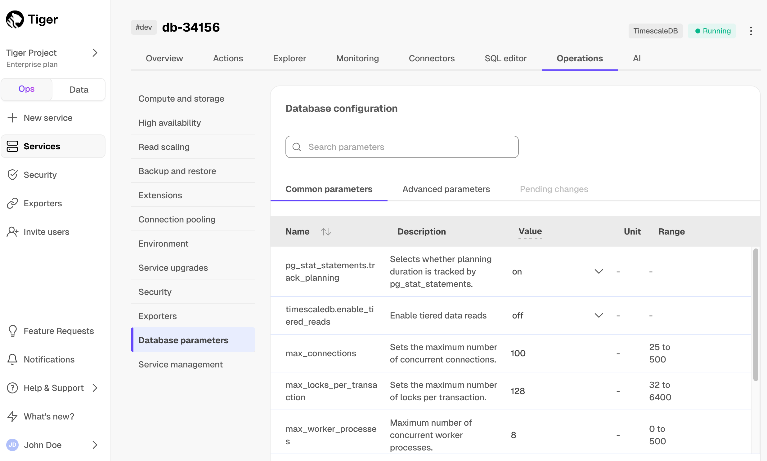
Modify basic parameters

Under the Common parameters tab, you can modify a limited set of the parameters that are most often modified in a Tiger Cloud or Postgres instance. To modify a configured value, hover over the value and click the revealed pencil icon. This reveals an editable field to apply your change. Clicking anywhere outside of that field saves the value to be applied.

Apply configuration changes

When you have modified the configuration parameters that you would like to change, click Apply changes. For some changes, such as timescaledb.max_background_workers, the service needs to be restarted. In this case, the button reads Apply changes and restart.

A confirmation dialog is displayed which indicates whether a restart is required. Click Confirm to apply the changes, and restart if necessary.

===== PAGE: https://docs.tigerdata.com/use-timescale/configuration/advanced-parameters/ =====

Advanced parameters

It is possible to configure a wide variety of Tiger Cloud service database parameters by navigating to the Advanced parameters tab under the Database configuration heading. The advanced parameters are displayed in a scrollable and searchable list.

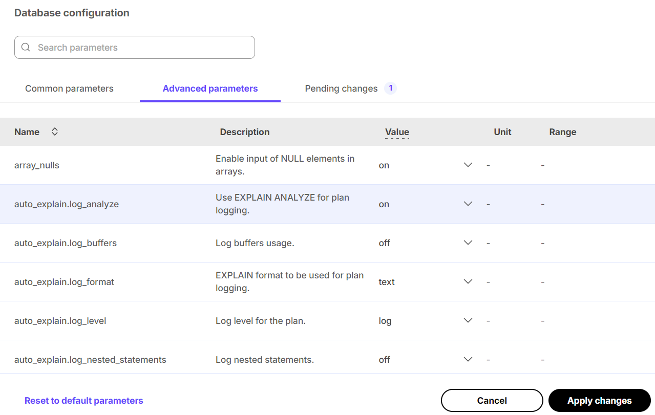
As with the basic database configuration parameters, any changes are highlighted and the Apply changes, or Apply changes and restart, button is available, prompting you to confirm changes before the service is modified.

Multiple databases

To create more than one database, you need to create a new service for each database. Tiger Cloud does not support multiple databases within the same service. Having a separate service for each database affords each database its own isolated resources.

You can also use [schemas][schemas] to organize tables into logical groups. A single database can contain multiple schemas, which in turn contain tables. The main difference between isolating with databases versus schemas is that a user can access objects in any of the schemas in the database they are connected to, so long as they have the corresponding privileges. Schemas can help isolate smaller use cases that do not warrant their own service.

Please refer to the [Grand Unified Configuration (GUC) parameters][gucs] for a complete list.

Policies

`timescaledb.max_background_workers (int)`

Max background worker processes allocated to TimescaleDB. Set to at least 1 + the number of databases loaded with the TimescaleDB extension in a Postgres instance. Default value is 16.

Tiger Cloud service tuning

`timescaledb.disable_load (bool)`

Disable the loading of the actual extension

===== PAGE: https://docs.tigerdata.com/use-timescale/ha-replicas/read-scaling/ =====

Read scaling

When read-intensive workloads compete with high ingest rates, your primary data instance can become a bottleneck. Spiky query traffic, analytical dashboards, and business intelligence tools risk slowing down ingest performance and disrupting critical write operations.

With read replica sets in Tiger Cloud, you can scale reads horizontally and keep your applications responsive. By offloading queries to replicas, your service maintains high ingest throughput while serving large or unpredictable read traffic with ease. This approach not only protects write performance but also gives you confidence that your read-heavy apps and BI workloads will run smoothly—even under pressure.

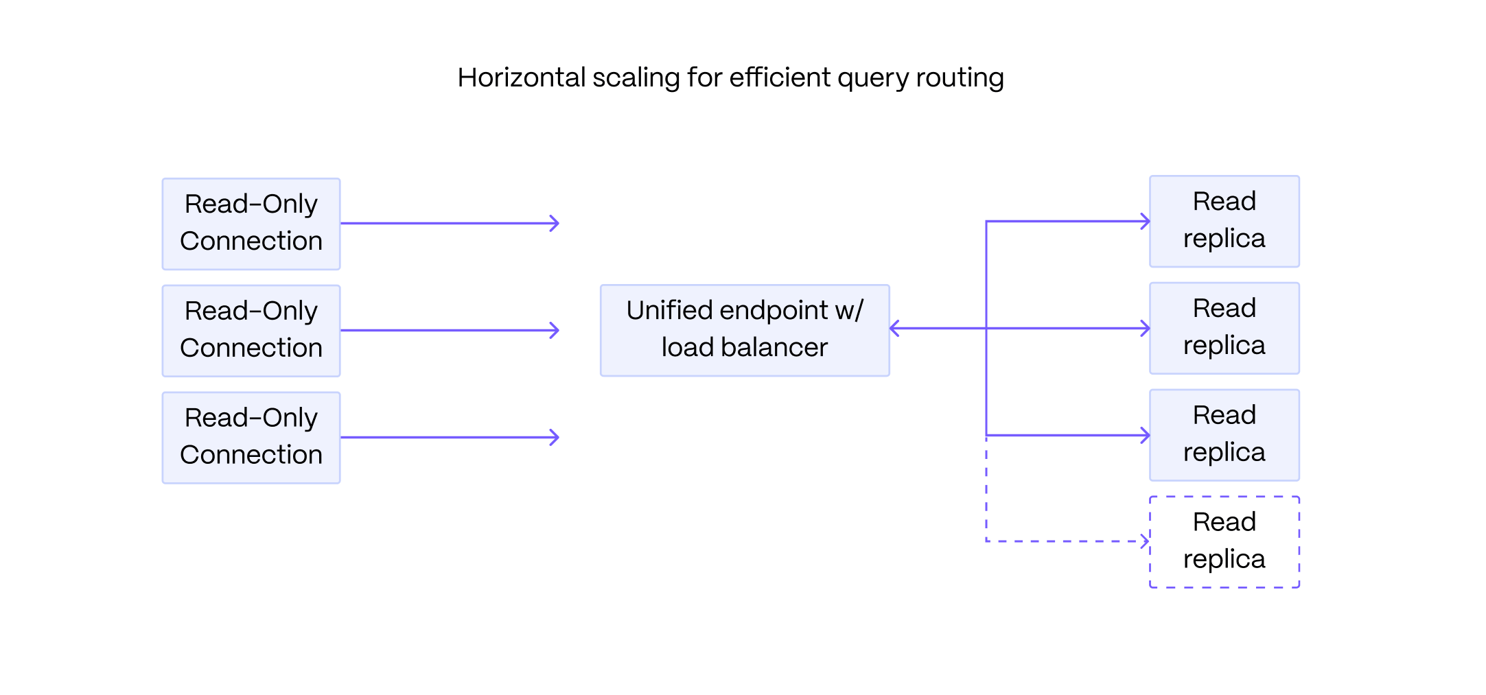
This page shows you how to create and manage read replica sets in Tiger Cloud Console.

What is read replication?

A read replica is a read-only copy of your primary database instance. Queries on read replicas have minimal impact on the performance of the primary instance. This enables you to interact with up-to-date production data for analysis, or to scale out reads beyond the limits of your primary instance. Read replicas can be short-lived and deleted when a session of data analysis is complete, or long-running to power an application or a business intelligence tool.

A read replica set in Tiger Cloud is a group of one or more read replica nodes that are accessed through the same endpoint. You query each set as a single replica. Tiger Cloud balances the load between the nodes in the set for you.

You can create as many read replica sets as you need. For security and resource isolation, each read replica set has unique connection details.

You use read replica sets for horizontal read scaling. To limit data loss for your Tiger Cloud services, use [high-availability replicas][ha].

Prerequisites

To follow this procedure:

Create a target Tiger Cloud service.
Create a [read-only user][read-only-role] on the primary data instance.
A user with read-only permissions cannot make changes in the primary database. This user is propagated to the read replica set when you create it.

Create a read replica set

To create a secure read replica set for your read-intensive apps:

In [Tiger Cloud Console][timescale-console-services], select your target service
Click Operations > Read scaling > Add a read replica set
Configure your replica set
Configure the number of nodes, compute size, connection pooling, and the name for your replica, then click Create read replica set.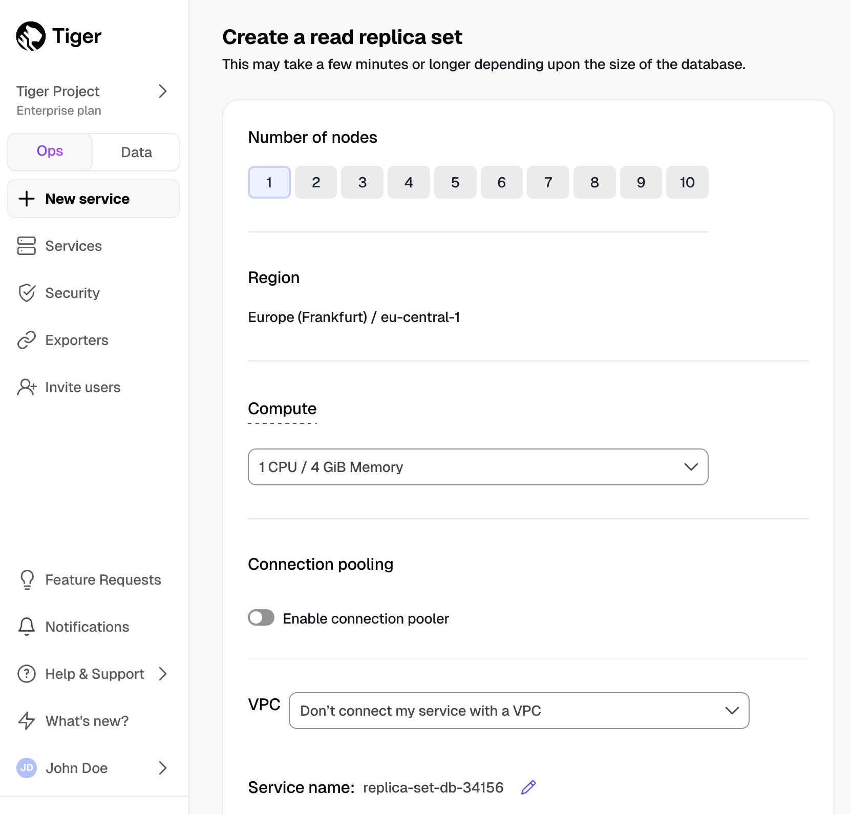
Save the connection information
The username and password of a read replica set are the same as the primary service. They cannot be changed independently.
The connection information for each read replica set is unique. You can add or remove nodes from an existing set and the connection information of that set will remain the same. To find the connection information for an existing read replica set:
1. Select the primary service in Tiger Cloud Console.
2. Click Operations > Read scaling.
3. Click the 🔗 icon next to the replica set in the list.

Edit a read replica set

You can edit an existing read replica set to better handle your reads. This includes changing the number of nodes, compute size, storage, and IOPS, as well as configuring VPC and other features.

To change the compute and storage configuration of your read replica set:

In [Tiger Cloud Console][timescale-console-services], expand and click the read replica set under your primary service
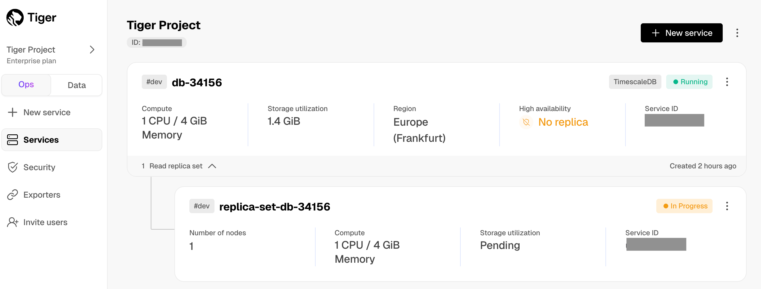
Click Operations > Compute and storage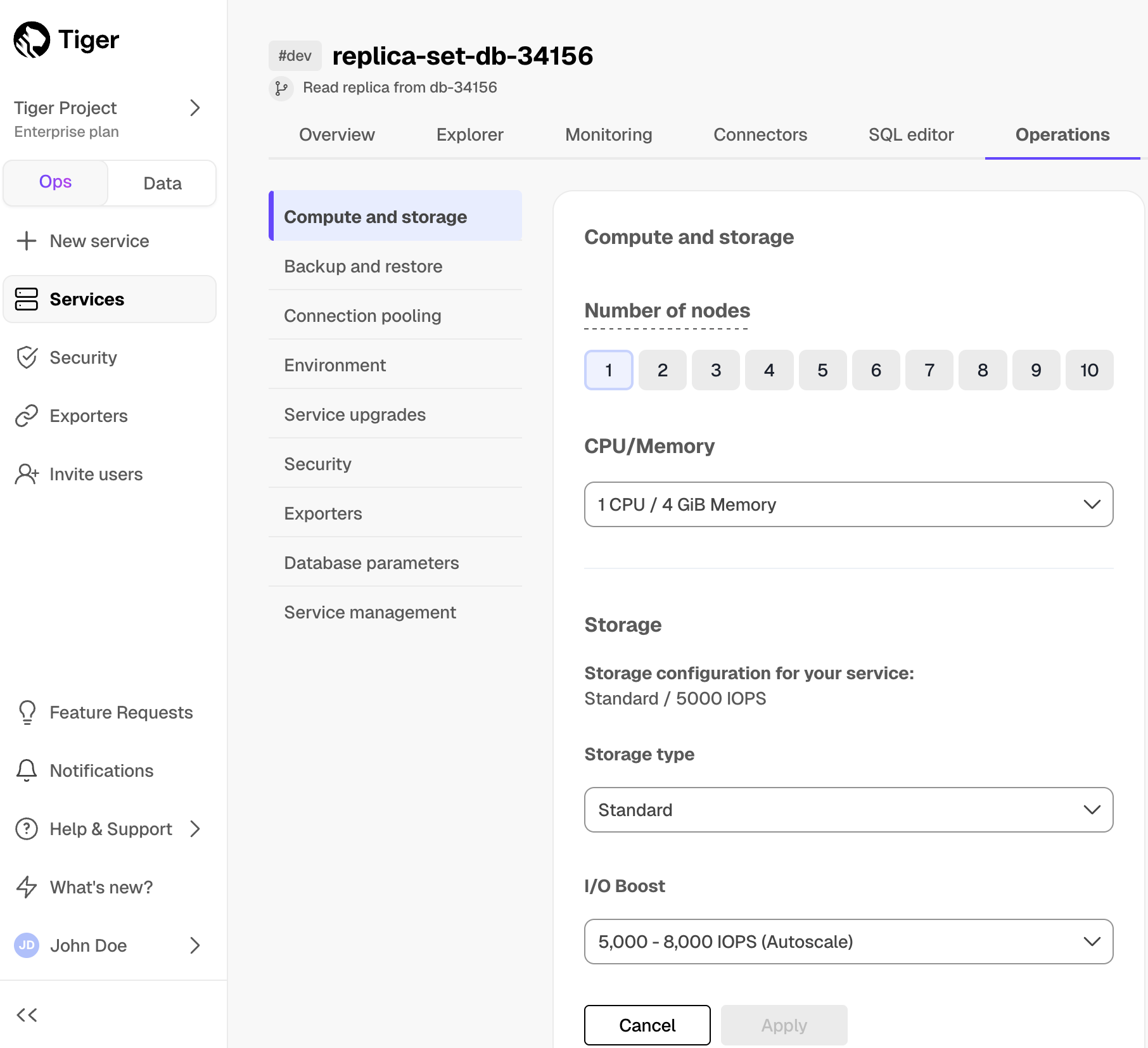
Change the replica configuration and click Apply

Manage data lag for your read replica sets

Read replica sets use asynchronous replication. This can cause a slight lag in data to the primary database instance. The lag is measured in bytes, against the current state of the primary instance. To check the status and lag for your read replica set:

In [Tiger Cloud Console][timescale-console-services], select your primary service
Click Operations > Read scaling
You see a list of configured read replica sets for this service, including their status and lag:
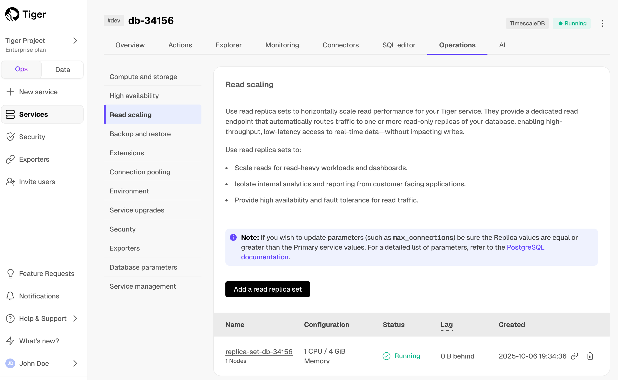
Configure the allowable lag
1. Select the replica set in the list.
2. Click Operations > Database parameters.
3. Adjust max_standby_streaming_delay and max_standby_archive_delay.
  This is not recommended for cases where changes must be immediately represented, for example, for user credentials.

Delete a read replica set

To delete a replica set:

In [Tiger Cloud Console][timescale-console-services], select your primary service
Click Operations > Read scaling
Click the trash icon next to a replica set
Confirm the deletion when prompted.

===== PAGE: https://docs.tigerdata.com/use-timescale/ha-replicas/high-availability/ =====

Manage high availability

For Tiger Cloud services where every second of uptime matters, Tiger Cloud delivers High Availability (HA) replicas. These replicas safeguard your data and keep your service running smoothly, even in the face of unexpected failures. By minimizing downtime and protecting against data loss, HA replicas ensure business continuity and give you the confidence to operate without interruption, including during routine maintenance.

This page shows you how to choose the best high availability option for your service.

What is HA replication?

HA replicas are exact, up-to-date copies of your database hosted in multiple AWS availability zones (AZ) within the same region as your primary node. They automatically take over operations if the original primary data node becomes unavailable. The primary node streams its write-ahead log (WAL) to the replicas to minimize the chances of data loss during failover.

HA replicas can be synchronous and asynchronous.

Synchronous: the primary commits its next write once the replica confirms that the previous write is complete. There is no lag between the primary and the replica. They are in the same state at all times. This is preferable if you need the highest level of data integrity. However, this affects the primary ingestion time.
Asynchronous: the primary commits its next write without the confirmation of the previous write completion. The asynchronous HA replicas often have a lag, in both time and data, compared to the primary. This is preferable if you need the shortest primary ingest time.

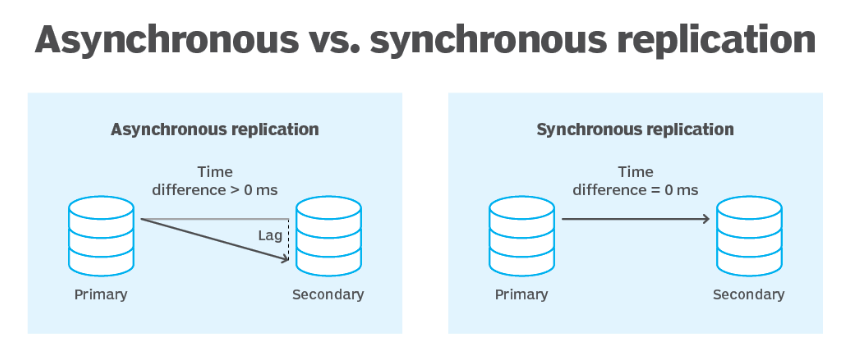
HA replicas have separate unique addresses that you can use to serve read-only requests in parallel to your primary data node. When your primary data node fails, Tiger Cloud automatically fails over to an HA replica within 30 seconds. During failover, the read-only address is unavailable while Tiger Cloud automatically creates a new HA replica. The time to make this replica depends on several factors, including the size of your data.

Operations such as upgrading your service to a new major or minor version may necessitate a service restart. Restarts are run during the [maintenance window][upgrade]. To avoid any downtime, each data node is updated in turn. That is, while the primary data node is updated, a replica is promoted to primary. After the primary is updated and online, the same maintenance is performed on the HA replicas.

To ensure that all services have minimum downtime and data loss in the most common failure scenarios and during maintenance, [rapid recovery][rapid-recovery] is enabled by default for all services.

Choose an HA strategy

The following HA configurations are available in Tiger Cloud:

Non-production: no replica, best for developer environments.
High availability: a single async replica in a different AWS availability zone from your primary. Provides high availability with cost efficiency. Best for production apps.
Highest availability: two replicas in different AWS availability zones from your primary. Available replication modes are:
- High performance - two async replicas. Provides the highest level of availability with two AZs and the ability to query the HA system. Best for apps where service availability is most critical.
- High data integrity - one sync replica and one async replica. The sync replica is identical to the primary at all times. Best for apps that can tolerate no data loss.

The following table summarizes the differences between these HA configurations:

	High availability (1 async)	High performance (2 async)	High data integrity (1 sync + 1 async)
Write flow	The primary streams its WAL to the async replica, which may have a slight lag compared to the primary, providing 99.9% uptime SLA.	The primary streams its writes to both async replicas, providing 99.9+% uptime SLA.	The primary streams its writes to the sync and async replicas. The async replica is never ahead of the sync one.
Additional read replica	Recommended. Reads from the HA replica may cause availability and lag issues.	Not needed. You can still read from the HA replica even if one of them is down. Configure an additional read replica only if your read use case is significantly different from your write use case.	Highly recommended. If you run heavy queries on a sync replica, it may fall behind the primary. Specifically, if it takes too long for the replica to confirm a transaction, the next transaction is canceled.
Choosing the replica to read from manually	Not applicable.	Not available. Queries are load-balanced against all available HA replicas.	Not available. Queries are load-balanced against all available HA replicas.
Sync replication	Only async replicas are supported in this configuration.	Only async replicas are supported in this configuration.	Supported.
Failover flow	<ul><li>If the primary fails, the replica becomes the primary while a new node is created, with only seconds of downtime.</li><li>If the replica fails, a new async replica is created without impacting the primary. If you read from the async HA replica, those reads fail until the new replica is available.</li></ul>	<ul><li>If the primary fails, one of the replicas becomes the primary while a new node is created, with the other one still available for reads.</li><li>If the replica fails, a new async replica is created in another AZ, without impacting the primary. The newly created replica is behind the primary and the original replica while it catches up.</li></ul>	<ul><li>If the primary fails, the sync replica becomes the primary while a new node is created, with the async one still available for reads.</li><li>If the async replica fails, a new async replica is created. Heavy reads on the sync replica may delay the ingest time of the primary while a new async replica is created. Data integrity remains high but primary ingest performance may degrade.</li><li>If the sync replica fails, the async replica becomes the sync one, and a new async replica is created. The primary may experience some ingest performance degradation during this time.</li></ul>
Cost composition	Primary + async (2x)	Primary + 2 async (3x)	Primary + 1 async + 1 sync (3x)
Tier	Performance, Scale, and Enterprise	Scale and Enterprise	Scale and Enterprise

The High and Highest HA strategies are available with the [Scale and the Enterprise][pricing-plans] pricing plans.

To enable HA for a service:

In [Tiger Cloud Console][cloud-login], select the service to enable replication for.
Click Operations, then select High availability.
Choose your replication strategy, then click Change configuration.
In Change high availability configuration, click Change config.

To change your HA replica strategy, click Change configuration, choose a strategy and click Change configuration. To download the connection information for the HA replica, either click the link next to the replica Active configuration, or find the information in the Overview tab for this service.

Test failover for your HA replicas

To test the failover mechanism, you can trigger a switchover. A switchover is a safe operation that attempts a failover, and throws an error if the replica or primary is not in a state to safely switch.

Connect to your primary node as tsdbadmin or another user that is part of the tsdbowner group.
You can also connect to the HA replica and check its node using this procedure.
At the psql prompt, connect to the postgres database:
sql
```
\c postgres
```
You should see postgres=> prompt.
Check if your node is currently in recovery:
sql
```
select pg_is_in_recovery();
```
Check which node is currently your primary:
sql
```
select * from pg_stat_replication;
```
Note the application_name. This is your service ID followed by the node. The important part is the -an-0 or -an-1.
Schedule a switchover:
sql
```
CALL tscloud.cluster_switchover();
```
By default, the switchover occurs in 30 secs. You can change the time by passing an interval, like this:
sql
```
CALL tscloud.cluster_switchover('15 seconds'::INTERVAL);
```

Wait for the switchover to occur, then check which node is your primary:

sql

SELECT * FROM pg_stat_replication;

You should see a notice that your connection has been reset, like this:

sql

FATAL:  terminating connection due to administrator command
SSL connection has been closed unexpectedly
The connection to the server was lost. Attempting reset: Succeeded.

Check the application_name. If your primary was -an-1 before, it should now be -an-0. If it was -an-0, it should now be -an-1.

===== PAGE: https://docs.tigerdata.com/use-timescale/data-tiering/tiered-data-replicas-forks/ =====

Replicas and forks with tiered data

There is one more thing that makes Tiered Storage even more amazing: when you keep data in the low-cost object storage tier, you pay for this data only once, regardless of whether you have a [high-availability replica][ha-replica] or [read replicas][read-replica] running in your service. We call this the savings multiplication effect of Tiered Storage.

The same applies to [forks][operations-forking], which you can use, for example, for running tests or creating dev environments. When creating one (or more) forks, you won't be billed for data shared with the primary in the low-cost storage.

If you decide to tier more data that's not in the primary, you will pay to store it in the low-cost tier, but you will still see substantial savings by moving that data from the high-performance tier of the fork to the cheaper object storage tier.

How this works behind the scenes

Once you tier data to the low-cost object storage tier, we keep a reference to that data on your Database's catalog.

Creating a replica or forking a primary server only copies the references and the metadata we keep on the catalog for all tiered data.

On the billing side, we only count and bill once for the data tiered, not for each reference there may exist towards that data.

What happens when a chunk is dropped or untiered on a fork

Dropping or untiering a chunk from a fork does not delete it from any other servers that reference the same chunk.

You can have one, multiple or 0 servers referencing the same chunk of data:

That means that deleting data from a fork does not affect the other servers (including the primary); it just removes the reference to that data, which is for all intends and purposes equal to deleting that data from the point of view of that fork
The primary and other servers are unaffected, as they still have their references and the metadata on their catalogs intact
We never delete anything on the object storage tier if at least one server references it: The data is only permanently deleted (or hard deleted as we internally call this operation) once the references drop to 0

As described above, tiered chunks are only counted once for billing purposes, so dropping or untiering a chunk that is shared with other servers from a fork will not affect billing as it was never counted for billing purposes.

Droping or untiering a chunk that was only tiered on that fork works as expected and is covered in more detail in the following section.

What happens when a chunk is modified on a fork

As a reminder, tiered data is immutable - there is no such thing as updating the data.

You can untier or drop a chunk, in which case what is described in the previous section covers what happens.

And you can tier new data, at which point a fork deviates from the primary in a similar way as all forks do.

New data tiered are not shared with parent or sibling servers, this is new data tiered for that server and we count them as a new object for the purposes of billing.

Similar to other types of storage tiers, this type of deviation can not happen for replicas as they have to be identical with the primary server, that's why we don't mention replicas when discussing about droping chunks or tiering additional data.

What happens with backups and PITR

As discussed above, we never delete anything on the object storage tier if at least one server references it. The data is only permanently deleted (or hard deleted as we internally call this operation) once the references drop to 0.

In addition to that, we delay hard deleting the data by 14 days, so that in case of a restore or PITR, all tiered data will be available. In the case of such a restore, new references are added to the deleted tiered chunks, so they are not any more candidates for a hard deletion.

Once 14 days pass after soft deleting the data,that is the number of references to the tiered data drop to 0, we hard delete the tiered data.

===== PAGE: https://docs.tigerdata.com/use-timescale/data-tiering/enabling-data-tiering/ =====

Manage storage and tiering

The tiered storage architecture in Tiger Cloud includes a high-performance storage tier and a low-cost object storage tier:

You use [high-performance storage][high-performance-storage] to store and query frequently accessed data.
You use [low-cost object storage][low-cost-storage] to cut costs by migrating rarely used data from the high-performance storage. After you enable tiered storage, you then either [create automated tiering policies][tiering-policies] or [manually tier and untier data][manual-tier].

You can query the data on the object storage tier, but you cannot modify it. Make sure that you are not tiering data that needs to be actively modified.

For low-cost storage, Tiger Data charges only for the size of your data in S3 in the Apache Parquet format, regardless of whether it was compressed in Tiger Cloud before tiering. There are no additional expenses, such as data transfer or compute.

High-performance storage tier

By default, Tiger Cloud stores your service data in the standard high-performance storage. This storage tier comes in the standard and enhanced types. Enhanced storage is available under the [Enterprise pricing plan][pricing-plans] only.

Standard high-performance storage

This storage type gives you up to 16 TB of storage and is available under [all pricing plans][pricing-plans]. You change the IOPS value to better suit your needs in Tiger Cloud Console:

In [Tiger Cloud Console][console], select your service, then click Operations > Compute and storage
By default, the type of high-performance storage is set to Standard.
Select the IOPS value in the I/O boost dropdown
- Under the [Performance pricing plan][pricing-plans], IOPS is set to 3,000 - 5,000 autoscale and cannot be changed.
- Under the [Scale and Enterprise pricing plans][pricing-plans], IOPS is set to 5,000 - 8,000 autoscale and can be upgraded to 16,000 IOPS.
Click Apply

Enhanced high-performance storage

This storage type gives you up to 64 TB and 32,000 IOPS, and is available under the [Enterprise pricing plan][pricing-plans]. To get enhanced storage:

In [Tiger Cloud Console][console], select your service, then click Operations > Compute and storage
Select Enhanced in the Storage type dropdown
The enhanced storage is currently not available in sa-east-1.
Select the IOPS value in the I/O boost dropdown
Select between 8,000, 16,000, 24,000, and 32,0000 IOPS. The value that you can apply depends on the number of CPUs in your service. Tiger Cloud Console notifies you if your selected IOPS requires increasing the number of CPUs. To increase IOPS to 64,000, click Contact us and we will be in touch to confirm the details.
Click Apply

You change from enhanced storage to standard in the same way. If you are using over 16 TB of enhanced storage, changing back to standard is not available until you shrink your data to be under 16 TB. You can make changes to the storage type and I/O boost settings without any downtime. Wait at least 6 hours to attempt another change.

Low-cost object storage tier

You enable the low-cost object storage tier in Tiger Cloud Console and then tier the data with policies or manually.

Enable tiered storage

You enable tiered storage from the Overview tab in Tiger Cloud Console.

In [Tiger Cloud Console][console], select the service to modify
In Explorer, click Storage configuration > Tiering storage, then click Enable tiered storage
Once enabled, you can proceed to [tier data manually][manual-tier] or [set up tiering policies][tiering-policies]. When tiered storage is enabled, you see the amount of data in the tiered object storage.

Automate tiering with policies

A tiering policy automatically moves any chunks that only contain data older than the move_after threshold to the object storage tier. This works similarly to a [data retention policy][data-retention], but chunks are moved rather than deleted.

A tiering policy schedules a job that runs periodically to asynchronously migrate eligible chunks to object storage. Chunks are considered tiered once they appear in the timescaledb_osm.tiered_chunks view.

You can add tiering policies to [hypertables][hypertable], including [continuous aggregates][caggs]. To manage tiering policies, [connect to your service][connect-to-service] and run the queries below in the data mode, the SQL editor, or using psql.

📂 提示词分类 - 软件工程，vibe coding用提示词（基于Excel原始数据)

Ccxt Documentation Index

Claude Cookbooks

Skills

Coingecko Documentation Index

Cryptocurrency Exchange Feed Handler

Hummingbot Documentation Index

Real time data client

Postgresql Documentation Index

Proxychains 参考文档索引

references

Telegram 生态开发资源索引

Timescaledb Documentation Index

twscrape Reference Documentation

add_dimension() ​

Samples ​

Parallelizing queries across multiple data nodes ​

Parallelizing disk I/O on a single node ​

Required arguments ​

Optional arguments ​

Returns ​

hypertable_approximate_detailed_size() ​

Samples ​

Required arguments ​

Returns ​

set_integer_now_fun() ​

Samples ​

Required arguments ​

Optional arguments ​

CREATE INDEX (Transaction Per Chunk) ​

Samples ​

refresh_continuous_aggregate() ​

Samples ​

Required arguments ​

Optional arguments ​

remove_policies() ​

Samples ​

Required arguments ​

Optional arguments ​

Returns ​

add_continuous_aggregate_policy() ​

Samples ​

Required arguments ​

Optional arguments ​

Returns ​

hypertable_size() ​

hypertable_size() ​

Samples ​

Required arguments ​

Returns ​

alter_policies() ​

Samples ​

Required arguments ​

Optional arguments ​

Returns ​

remove_continuous_aggregate_policy() ​

Samples ​

Required arguments ​

Optional arguments ​

add_policies() ​

Samples ​

Required arguments ​

Optional arguments ​

Returns ​

CREATE MATERIALIZED VIEW (Continuous Aggregate) ​

Samples ​

Parameters ​

ALTER MATERIALIZED VIEW (Continuous Aggregate) ​

Samples ​

Arguments ​

cagg_migrate() ​

Required arguments ​

Optional arguments ​

DROP MATERIALIZED VIEW (Continuous Aggregate) ​

Samples ​

Parameters ​

remove_all_policies() ​

Samples ​

Required arguments ​

Optional arguments ​

add_dimension()

Samples

Parallelizing queries across multiple data nodes

Parallelizing disk I/O on a single node

Required arguments

Optional arguments

Returns

hypertable_approximate_detailed_size()

Samples

Required arguments

Returns

set_integer_now_fun()

Samples

Required arguments

Optional arguments

CREATE INDEX (Transaction Per Chunk)

Samples

refresh_continuous_aggregate()

Samples

Required arguments

Optional arguments

remove_policies()

Samples

Required arguments

Optional arguments

Returns

add_continuous_aggregate_policy()

Samples

Required arguments

Optional arguments

Returns

hypertable_size()

hypertable_size()

Samples

Required arguments

Returns

alter_policies()

Samples

Required arguments

Optional arguments

Returns

remove_continuous_aggregate_policy()

Samples

Required arguments

Optional arguments

add_policies()

Samples

Required arguments

Optional arguments

Returns

CREATE MATERIALIZED VIEW (Continuous Aggregate)

Samples

Parameters

ALTER MATERIALIZED VIEW (Continuous Aggregate)

Samples

Arguments

cagg_migrate()

Required arguments

Optional arguments

DROP MATERIALIZED VIEW (Continuous Aggregate)

Samples

Parameters

remove_all_policies()

Samples

Required arguments

Optional arguments

Returns

hypertable_detailed_size()

hypertable_detailed_size()

Samples

Required arguments

Returns

show_policies()

Samples

Required arguments

Returns

ALTER TABLE (hypercore)

Samples

Arguments

chunk_columnstore_stats()