3.1 Language Models and Transformer Architecture

3.1.1 From N-gram to RNN

Language Model (LM) is the core of natural language processing, and its fundamental task is to calculate the probability of a word sequence (i.e., a sentence) appearing. A good language model can tell us what kind of sentences are fluent and natural. In multi-agent systems, language models are the foundation for agents to understand human instructions and generate responses. This section will review the evolution from classical statistical methods to modern deep learning models, laying a solid foundation for understanding the subsequent Transformer architecture.

(1) Statistical Language Models and the N-gram Idea

Before the rise of deep learning, statistical methods were the mainstream of language models. The core idea is that the probability of a sentence appearing equals the product of the conditional probabilities of each word in the sentence. For a sentence S composed of words $w_1,w_2,\cdots,w_m$, its probability P(S) can be expressed as:

$$P(S)=P(w_1,w_2,…,w_m)=P(w_1)⋅P(w_2∣w_1)⋅P(w_3∣w_1,w_2)⋯P(w_m∣w_1,…,w_{m−1})$$

This formula is called the chain rule of probability. However, directly calculating this formula is almost impossible because conditional probabilities like $P(w_m∣w_1,\cdots,w_{m−1})$ are too difficult to estimate from a corpus, as the word sequence $w_1,\cdots,w_{m−1}$ may have never appeared in the training data.

Figure 3.1 Schematic diagram of Markov assumption

To solve this problem, researchers introduced the Markov Assumption. Its core idea is: we don't need to trace back a word's entire history; we can approximately assume that a word's probability of appearing is only related to the limited $n−1$ words before it, as shown in Figure 3.1. Language models built on this assumption are called N-gram models. Here, "N" represents the context window size we consider. Let's look at some of the most common examples to understand this concept:

• Bigram (when N=2): This is the simplest case, where we assume a word's appearance is only related to the one word before it. Therefore, the complex conditional probability $P(w_i∣w_1,\cdots,w_{i−1})$ in the chain rule can be approximated to a more easily calculable form:

$$P(w_{i}∣w_{1},…,w_{i−1})≈P(w_{i}∣w_{i−1})$$

• Trigram (when N=3): Similarly, we assume a word's appearance is only related to the two words before it:

$$P(w_i∣w_1,…,w_{i−1})≈P(w_i∣w_{i−2},w_{i−1})$$

These probabilities can be calculated through Maximum Likelihood Estimation (MLE) in large corpora. This term sounds complex, but its idea is very intuitive: what is most likely to appear is what we see most often in the data. For example, for a Bigram model, we want to calculate the probability $P(w_i∣w_{i−1})$ that the next word is $w_i$ after word $w_{i−1}$ appears. According to maximum likelihood estimation, this probability can be estimated through simple counting:

$$P(w_i∣w_{i−1})=\frac{Count(w_{i−1},w_i)}{Count(w_{i−1})}$$

Here, the Count() function represents "counting":

• $Count(w_{i−1},w_i)$: represents the total number of times the word pair $(w_{i−1},w_i)$ appears consecutively in the corpus.
• $Count(w_{i−1})$: represents the total number of times the single word $w_{i−1}$ appears in the corpus.

The formula's meaning is: we use "the number of times word pair $Count(w_{i−1},w_i)$ appears" divided by "the total number of times word $Count(w_{i−1})$ appears" as an approximate estimate of $P(w_i∣w_{i−1})$.

To make this process more concrete, let's manually perform a calculation. Suppose we have a mini corpus containing only the following two sentences: datawhale agent learns, datawhale agent works. Our goal is: using a Bigram (N=2) model, estimate the probability of the sentence datawhale agent learns appearing. According to the Bigram assumption, we examine consecutive pairs of words (i.e., word pairs) each time.

Step 1: Calculate the probability of the first word $P(datawhale)$ This is the number of times datawhale appears divided by the total number of words. datawhale appears 2 times, and the total number of words is 6.

$$P(\text{datawhale}) = \frac{\text{Number of "datawhale" in total corpus}}{\text{Total number of words in corpus}} = \frac{2}{6} \approx 0.333$$

Step 2: Calculate conditional probability $P(agent∣datawhale)$ This is the number of times the word pair datawhale agent appears divided by the total number of times datawhale appears. datawhale agent appears 2 times, datawhale appears 2 times.

$$P(\text{agent}|\text{datawhale}) = \frac{\text{Count}(\text{datawhale agent})}{\text{Count}(\text{datawhale})} = \frac{2}{2} = 1$$

Step 3: Calculate conditional probability $P(learns∣agent)$ This is the number of times the word pair agent learns appears divided by the total number of times agent appears. agent learns appears 1 time, agent appears 2 times.

$$P(\text{learns}|\text{agent}) = \frac{\text{Count(agent learns)}}{\text{Count(agent)}} = \frac{1}{2} = 0.5$$

Finally: Multiply the probabilities So, the approximate probability of the entire sentence is:

$$P(\text{datawhale agent learns}) \approx P(\text{datawhale}) \cdot P(\text{agent}|\text{datawhale}) \cdot P(\text{learns}|\text{agent}) \approx 0.333 \cdot 1 \cdot 0.5 \approx 0.167$$

import collections

# Example corpus, consistent with the corpus in the case explanation above
corpus = "datawhale agent learns datawhale agent works"
tokens = corpus.split()
total_tokens = len(tokens)

# --- Step 1: Calculate P(datawhale) ---
count_datawhale = tokens.count('datawhale')
p_datawhale = count_datawhale / total_tokens
print(f"Step 1: P(datawhale) = {count_datawhale}/{total_tokens} = {p_datawhale:.3f}")

# --- Step 2: Calculate P(agent|datawhale) ---
# First calculate bigrams for subsequent steps
bigrams = zip(tokens, tokens[1:])
bigram_counts = collections.Counter(bigrams)
count_datawhale_agent = bigram_counts[('datawhale', 'agent')]
# count_datawhale was already calculated in step 1
p_agent_given_datawhale = count_datawhale_agent / count_datawhale
print(f"Step 2: P(agent|datawhale) = {count_datawhale_agent}/{count_datawhale} = {p_agent_given_datawhale:.3f}")

# --- Step 3: Calculate P(learns|agent) ---
count_agent_learns = bigram_counts[('agent', 'learns')]
count_agent = tokens.count('agent')
p_learns_given_agent = count_agent_learns / count_agent
print(f"Step 3: P(learns|agent) = {count_agent_learns}/{count_agent} = {p_learns_given_agent:.3f}")

# --- Finally: Multiply the probabilities ---
p_sentence = p_datawhale * p_agent_given_datawhale * p_learns_given_agent
print(f"Finally: P('datawhale agent learns') ≈ {p_datawhale:.3f} * {p_agent_given_datawhale:.3f} * {p_learns_given_agent:.3f} = {p_sentence:.3f}")

>>>
Step 1: P(datawhale) = 2/6 = 0.333
Step 2: P(agent|datawhale) = 2/2 = 1.000
Step 3: P(learns|agent) = 1/2 = 0.500
Finally: P('datawhale agent learns') ≈ 0.333 * 1.000 * 0.500 = 0.167

N-gram models, although simple and effective, have two fatal flaws:

1. Data Sparsity: If a word sequence has never appeared in the corpus, its probability estimate is 0, which is obviously unreasonable. Although this can be alleviated through smoothing techniques, it cannot be eradicated.
2. Poor Generalization Ability: The model cannot understand semantic similarity between words. For example, even if the model has seen agent learns many times in the corpus, it cannot generalize this knowledge to semantically similar words. When we calculate the probability of robot learns, if the word robot has never appeared, or if the combination robot learns has never appeared, the probability calculated by the model will also be zero. The model cannot understand the semantic similarity between agent and robot.

(2) Neural Network Language Models and Word Embeddings

The fundamental flaw of N-gram models is that they treat words as isolated, discrete symbols. To overcome this problem, researchers turned to neural networks and proposed an idea: represent words with continuous vectors. In 2003, the Feedforward Neural Network Language Model proposed by Bengio et al. was a milestone in this field^[1].

Its core idea can be divided into two steps:

1. Build a semantic space: Create a high-dimensional continuous vector space, then map each word in the vocabulary to a point in that space. This point (i.e., vector) is called a Word Embedding or word vector. In this space, semantically similar words have vectors that are close together in position. For example, the vectors of agent and robot will be very close, while the vectors of agent and apple will be far apart.
2. Learn the mapping from context to the next word: Utilize the powerful fitting ability of neural networks to learn a function. The input of this function is the word vectors of the previous $n−1$ words, and the output is the probability distribution of each word in the vocabulary appearing after the current context.

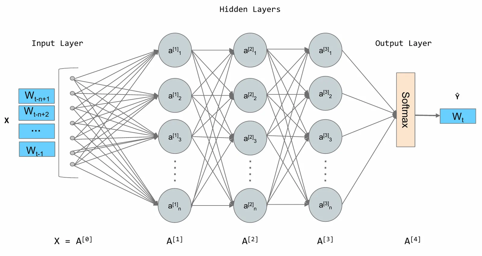
Figure 3.2 Schematic diagram of neural network language model architecture

As shown in Figure 3.2, in this architecture, word embeddings are automatically learned during model training. To complete the task of "predicting the next word," the model continuously adjusts the vector position of each word, ultimately making these vectors contain rich semantic information. Once we convert words into vectors, we can use mathematical tools to measure the relationships between them. The most commonly used method is Cosine Similarity, which measures their similarity by calculating the cosine of the angle between two vectors.

$$\text{similarity}(\vec{a}, \vec{b}) = \cos(\theta) = \frac{\vec{a} \cdot \vec{b}}{|\vec{a}| |\vec{b}|}$$

The meaning of this formula is:

• If two vectors have exactly the same direction, the angle is 0°, the cosine value is 1, indicating complete correlation.
• If two vectors are orthogonal, the angle is 90°, the cosine value is 0, indicating no relationship.
• If two vectors have completely opposite directions, the angle is 180°, the cosine value is -1, indicating complete negative correlation.

Through this method, word vectors can not only capture simple relationships like "synonyms" but also capture more complex analogical relationships.

A famous example demonstrates the semantic relationships captured by word vectors: vector('King') - vector('Man') + vector('Woman') The result of this vector operation is surprisingly close to the position of vector('Queen') in the vector space. This is like performing semantic translation: we start from the point "king," subtract the vector of "male," add the vector of "female," and finally arrive at the position of "queen." This proves that word embeddings can learn abstract concepts like "gender" and "royalty."

import numpy as np

# Assume we have learned simplified 2D word vectors
embeddings = {
    "king": np.array([0.9, 0.8]),
    "queen": np.array([0.9, 0.2]),
    "man": np.array([0.7, 0.9]),
    "woman": np.array([0.7, 0.3])
}

def cosine_similarity(vec1, vec2):
    dot_product = np.dot(vec1, vec2)
    norm_product = np.linalg.norm(vec1) * np.linalg.norm(vec2)
    return dot_product / norm_product

# king - man + woman
result_vec = embeddings["king"] - embeddings["man"] + embeddings["woman"]

# Calculate similarity between result vector and "queen"
sim = cosine_similarity(result_vec, embeddings["queen"])

print(f"Result vector of king - man + woman: {result_vec}")
print(f"Similarity of this result with 'queen': {sim:.4f}")

>>>
Result vector of king - man + woman: [0.9 0.2]
Similarity of this result with 'queen': 1.0000

Neural network language models successfully solved the poor generalization problem of N-gram models through word embeddings. However, they still have a limitation similar to N-gram: the context window is fixed. They can only consider a fixed number of preceding words, which laid the groundwork for recurrent neural networks that can handle sequences of arbitrary length.

(3) Recurrent Neural Networks (RNN) and Long Short-Term Memory Networks (LSTM)

Although the neural network language model in the previous section introduced word embeddings to solve the generalization problem, like N-gram models, its context window is of fixed size. To predict the next word, it can only see the previous n−1 words, and earlier historical information is discarded. This obviously does not conform to how we humans understand language. To break the limitation of fixed windows, Recurrent Neural Networks (RNN) emerged, with a very intuitive core idea: add "memory" capability to the network^[2].

As shown in Figure 3.3, RNN's design introduces a hidden state vector, which we can understand as the network's short-term memory. At each step of processing the sequence, the network reads the current input word and combines it with its memory from the previous moment (i.e., the hidden state from the previous time step), then generates a new memory (i.e., the hidden state of the current time step) to pass to the next moment. This cyclical process allows information to continuously propagate backward through the sequence.

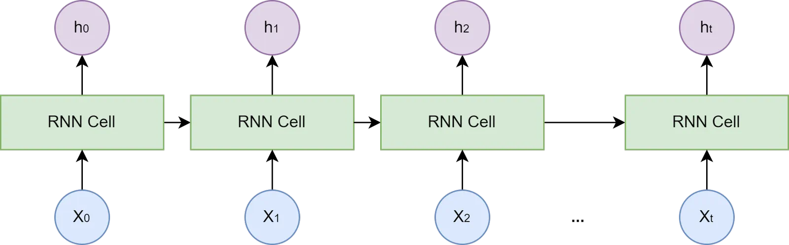
Figure 3.3 Schematic diagram of RNN structure

However, standard RNNs have a serious problem in practice: the Long-term Dependency Problem. During training, the model needs to adjust weights deep in the network based on errors at the output end through the backpropagation algorithm. For RNNs, the length of the sequence is the depth of the network. When the sequence is very long, gradients undergo multiple multiplications during backward propagation, which causes gradient values to rapidly approach zero (gradient vanishing) or become extremely large (gradient explosion). Gradient vanishing prevents the model from effectively learning the impact of early sequence information on later outputs, making it difficult to capture long-distance dependencies.

To solve the long-term dependency problem, Long Short-Term Memory (LSTM) was designed^[3]. LSTM is a special type of RNN, and its core innovation lies in introducing Cell State and a sophisticated Gating Mechanism. The cell state can be seen as an information pathway independent of the hidden state, allowing information to pass more smoothly between time steps. The gating mechanism consists of several small neural networks that can learn how to selectively let information through, thereby controlling the addition and removal of information in the cell state. These gates include:

• Forget Gate: Decides which information to discard from the cell state of the previous moment.
• Input Gate: Decides which new information from the current input to store in the cell state.
• Output Gate: Decides which information to output to the hidden state based on the current cell state.

3.1.2 Transformer Architecture Analysis

In the previous section, we saw that RNNs and LSTMs process sequential data by introducing recurrent structures, which to some extent solved the problem of capturing long-distance dependencies. However, this recurrent computation method also brought new bottlenecks: it must process data sequentially. The computation at time step t must wait for time step t−1 to complete before it can begin. This means RNNs cannot perform large-scale parallel computation and are inefficient when processing long sequences, which greatly limits the improvement of model scale and training speed. Transformer was proposed by the Google team in 2017^[4]. It completely abandoned the recurrent structure and instead relied entirely on a mechanism called Attention to capture dependencies within sequences, thereby achieving truly parallel computation.

(1) Overall Encoder-Decoder Structure

The original Transformer model was designed for the end-to-end task of machine translation. As shown in Figure 3.4, it follows a classic Encoder-Decoder architecture at the macro level.

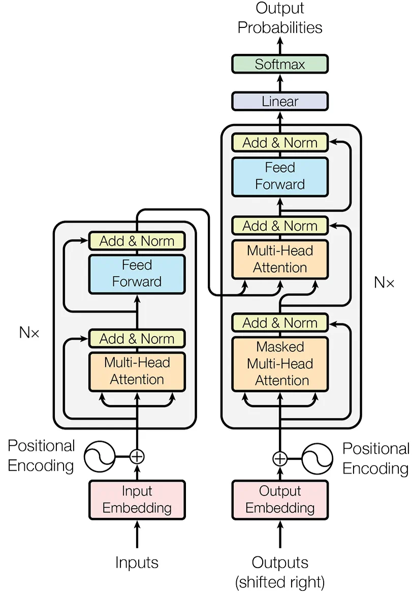
Figure 3.4 Overall Transformer architecture diagram

We can understand this structure as a team with clear division of labor:

1. Encoder: The task is to "understand" the entire input sentence. It reads all input tokens (this concept will be introduced in Section 3.2.2) and ultimately generates a vector representation rich in contextual information for each token.
2. Decoder: The task is to "generate" the target sentence. It references the preceding text it has already generated and "consults" the encoder's understanding results to generate the next word.

To truly understand how Transformer works, the best method is to implement it yourself. In this section, we will adopt a "top-down" approach: first, we build the complete code framework of Transformer, defining all necessary classes and methods. Then, like completing a puzzle, we will implement the specific functions of these classes one by one.

import torch
import torch.nn as nn
import math

# --- Placeholder modules, to be implemented in subsequent subsections ---

class PositionalEncoding(nn.Module):
    """
    Positional encoding module
    """
    def forward(self, x):
        pass

class MultiHeadAttention(nn.Module):
    """
    Multi-head attention mechanism module
    """
    def forward(self, query, key, value, mask):
        pass

class PositionWiseFeedForward(nn.Module):
    """
    Position-wise feed-forward network module
    """
    def forward(self, x):
        pass

# --- Encoder core layer ---

class EncoderLayer(nn.Module):
    def __init__(self, d_model, num_heads, d_ff, dropout):
        super(EncoderLayer, self).__init__()
        self.self_attn = MultiHeadAttention() # To be implemented
        self.feed_forward = PositionWiseFeedForward() # To be implemented
        self.norm1 = nn.LayerNorm(d_model)
        self.norm2 = nn.LayerNorm(d_model)
        self.dropout = nn.Dropout(dropout)

    def forward(self, x, mask):
        # Residual connection and layer normalization will be explained in detail in Section 3.1.2.4
        # 1. Multi-head self-attention
        attn_output = self.self_attn(x, x, x, mask)
        x = self.norm1(x + self.dropout(attn_output))

        # 2. Feed-forward network
        ff_output = self.feed_forward(x)
        x = self.norm2(x + self.dropout(ff_output))

        return x

# --- Decoder core layer ---

class DecoderLayer(nn.Module):
    def __init__(self, d_model, num_heads, d_ff, dropout):
        super(DecoderLayer, self).__init__()
        self.self_attn = MultiHeadAttention() # To be implemented
        self.cross_attn = MultiHeadAttention() # To be implemented
        self.feed_forward = PositionWiseFeedForward() # To be implemented
        self.norm1 = nn.LayerNorm(d_model)
        self.norm2 = nn.LayerNorm(d_model)
        self.norm3 = nn.LayerNorm(d_model)
        self.dropout = nn.Dropout(dropout)

    def forward(self, x, encoder_output, src_mask, tgt_mask):
        # 1. Masked multi-head self-attention (on itself)
        attn_output = self.self_attn(x, x, x, tgt_mask)
        x = self.norm1(x + self.dropout(attn_output))

        # 2. Cross-attention (on encoder output)
        cross_attn_output = self.cross_attn(x, encoder_output, encoder_output, src_mask)
        x = self.norm2(x + self.dropout(cross_attn_output))

        # 3. Feed-forward network
        ff_output = self.feed_forward(x)
        x = self.norm3(x + self.dropout(ff_output))

        return x

(2) From Self-Attention to Multi-Head Attention

Now, let's fill in the most critical module in the skeleton: the attention mechanism.

Imagine we are reading this sentence: "The agent learns because it is intelligent." When we read the bolded "it," to understand its reference, our brain unconsciously places more attention on the word "agent" earlier in the sentence. The Self-Attention mechanism is a mathematical modeling of this phenomenon. It allows the model to consider all other words in the sentence when processing each word and assign different "attention weights" to these words. The higher the weight of a word, the stronger its association with the current word, and the greater the proportion its information should occupy in the current word's representation.

To implement the above process, the self-attention mechanism introduces three learnable roles for each input token vector:

• Query (Q): Represents the current token, which is actively "querying" other tokens to obtain information.
• Key (K): Represents the "label" or "index" of tokens in the sentence that can be queried.
• Value (V): Represents the "content" or "information" carried by the token itself.

These three vectors are all obtained by multiplying the original word embedding vector by three different, learnable weight matrices ($W^Q,W^K,W^V$). The entire computation process can be divided into the following steps, which we can imagine as an efficient open-book exam:

• Prepare "exam questions" and "materials": For each word in the sentence, generate its $Q,K,V$ vectors through weight matrices.
• Calculate relevance scores: To calculate the new representation of word $A$, use word $A$'s $Q$ vector to perform dot product operations with the $K$ vectors of all words in the sentence (including $A$ itself). This score reflects the importance of other words for understanding word $A$.
• Stabilization and normalization: Divide all obtained scores by a scaling factor $\sqrt{d_{k}}$ ($d_{k}$ is the dimension of the $K$ vector) to prevent gradients from being too small, then use the Softmax function to convert scores into weights that sum to 1, which is the normalization process.
• Weighted sum: Multiply the weights obtained in the previous step by each word's corresponding $V$ vector, then add all results together. The final vector is the new representation of word $A$ after integrating global contextual information.

This process can be summarized by a concise formula:

$$\text{Attention}(Q,K,V)=\text{softmax}\left(\frac{QK^{T}}{\sqrt{d_{k}}}\right)V$$

If only one attention calculation is performed (i.e., single-head), the model may only learn to focus on one type of association. For example, when processing "it," it might only learn to focus on the subject. But relationships in language are complex, and we want the model to simultaneously focus on multiple relationships (such as referential relationships, tense relationships, subordinate relationships, etc.). Multi-head attention mechanism emerged. Its idea is simple: instead of doing it all at once, divide it into several groups, do them separately, then merge.

It splits the original Q, K, V vectors into h parts along the dimension (h is the number of "heads"), and each part independently performs a single-head attention calculation. This is like having h different "experts" examine the sentence from different perspectives, with each expert capturing a different feature relationship. Finally, the "opinions" (i.e., output vectors) of these h experts are concatenated, then integrated through a linear transformation to obtain the final output.

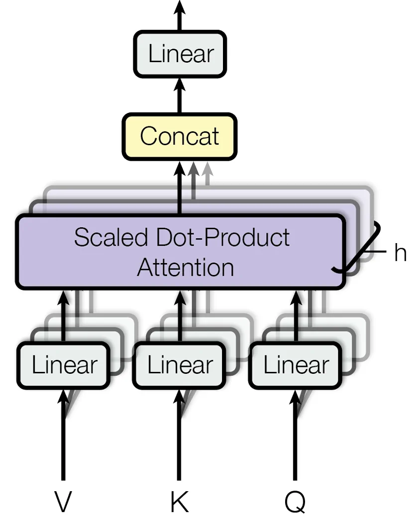
Figure 3.5 Multi-head attention mechanism

As shown in Figure 3.5, this design allows the model to jointly attend to information from different positions and different representation subspaces, greatly enhancing the model's expressive power. Below is a simple implementation of multi-head attention for reference.

class MultiHeadAttention(nn.Module):
    """
    Multi-head attention mechanism module
    """
    def __init__(self, d_model, num_heads):
        super(MultiHeadAttention, self).__init__()
        assert d_model % num_heads == 0, "d_model must be divisible by num_heads"

        self.d_model = d_model
        self.num_heads = num_heads
        self.d_k = d_model // num_heads

        # Define linear transformation layers for Q, K, V and output
        self.W_q = nn.Linear(d_model, d_model)
        self.W_k = nn.Linear(d_model, d_model)
        self.W_v = nn.Linear(d_model, d_model)
        self.W_o = nn.Linear(d_model, d_model)

    def scaled_dot_product_attention(self, Q, K, V, mask=None):
        # 1. Calculate attention scores (QK^T)
        attn_scores = torch.matmul(Q, K.transpose(-2, -1)) / math.sqrt(self.d_k)

        # 2. Apply mask (if provided)
        if mask is not None:
            # Set positions where mask is 0 to a very small negative number, so they approach 0 after softmax
            attn_scores = attn_scores.masked_fill(mask == 0, -1e9)

        # 3. Calculate attention weights (Softmax)
        attn_probs = torch.softmax(attn_scores, dim=-1)

        # 4. Weighted sum (weights * V)
        output = torch.matmul(attn_probs, V)
        return output

    def split_heads(self, x):
        # Transform input x shape from (batch_size, seq_length, d_model)
        # to (batch_size, num_heads, seq_length, d_k)
        batch_size, seq_length, d_model = x.size()
        return x.view(batch_size, seq_length, self.num_heads, self.d_k).transpose(1, 2)

    def combine_heads(self, x):
        # Transform input x shape from (batch_size, num_heads, seq_length, d_k)
        # back to (batch_size, seq_length, d_model)
        batch_size, num_heads, seq_length, d_k = x.size()
        return x.transpose(1, 2).contiguous().view(batch_size, seq_length, self.d_model)

    def forward(self, Q, K, V, mask=None):
        # 1. Perform linear transformations on Q, K, V
        Q = self.split_heads(self.W_q(Q))
        K = self.split_heads(self.W_k(K))
        V = self.split_heads(self.W_v(V))

        # 2. Calculate scaled dot-product attention
        attn_output = self.scaled_dot_product_attention(Q, K, V, mask)

        # 3. Combine multi-head outputs and perform final linear transformation
        output = self.W_o(self.combine_heads(attn_output))
        return output

(3) Feed-Forward Neural Network

In each Encoder and Decoder layer, the multi-head attention sublayer is followed by a Position-wise Feed-Forward Network (FFN). If the role of the attention layer is to "dynamically aggregate" relevant information from the entire sequence, then the role of the feed-forward network is to extract higher-order features from this aggregated information.

The key to this name is "position-wise." It means this feed-forward network acts independently on each token vector in the sequence. In other words, for a sequence of length seq_len, this FFN is actually called seq_len times, processing one token each time. Importantly, all positions share the same set of network weights. This design both maintains the ability to independently process each position and greatly reduces the model's parameter count. This network's structure is very simple, consisting of two linear transformations and a ReLU activation function:

$$\mathrm{FFN}(x)=\max\left(0, xW_{1}+b_{1}\right) W_{2}+b_{2}$$

Where $x$ is the output of the attention sublayer. $W_1,b_1,W_2,b_2$ are learnable parameters. Typically, the output dimension d_ff of the first linear layer is much larger than the input dimension d_model (for example, d_ff = 4 * d_model), then after ReLU activation, it is mapped back to d_model dimension through the second linear layer. This "expand then shrink" design is believed to help the model learn richer feature representations.

In our PyTorch skeleton, we can implement this module with the following code:

class PositionWiseFeedForward(nn.Module):
    """
    Position-wise feed-forward network module
    """
    def __init__(self, d_model, d_ff, dropout=0.1):
        super(PositionWiseFeedForward, self).__init__()
        self.linear1 = nn.Linear(d_model, d_ff)
        self.dropout = nn.Dropout(dropout)
        self.linear2 = nn.Linear(d_ff, d_model)
        self.relu = nn.ReLU()

    def forward(self, x):
        # x shape: (batch_size, seq_len, d_model)
        x = self.linear1(x)
        x = self.relu(x)
        x = self.dropout(x)
        x = self.linear2(x)
        # Final output shape: (batch_size, seq_len, d_model)
        return x

(4) Residual Connections and Layer Normalization

In each encoder and decoder layer of Transformer, all submodules (such as multi-head attention and feed-forward networks) are wrapped by an Add & Norm operation. This combination ensures that Transformer can train stably.

This operation consists of two parts:

• Residual Connection (Add): This operation directly adds the submodule's input x to the submodule's output Sublayer(x). This structure solves the Vanishing Gradients problem in deep neural networks. During backpropagation, gradients can bypass the submodule and propagate forward directly, ensuring that even if the network has many layers, the model can be effectively trained. Its formula can be expressed as: $\text{Output} = x + \text{Sublayer}(x)$.
• Layer Normalization (Norm): This operation normalizes all features of a single sample, making its mean 0 and variance 1. This solves the Internal Covariate Shift problem during model training, keeping the input distribution of each layer stable, thereby accelerating model convergence and improving training stability.

3.1.2.5 Positional Encoding

We already understand that the core of Transformer is the self-attention mechanism, which captures dependencies by calculating relationships between any two tokens in a sequence. However, this computation method has an inherent problem: it does not contain any information about token order or position. For self-attention, the two sequences "agent learns" and "learns agent" are completely equivalent because it only cares about relationships between tokens and ignores their arrangement. To solve this problem, Transformer introduced Positional Encoding.

The core idea of positional encoding is to add an additional "position vector" representing its absolute and relative position information to each token embedding vector in the input sequence. This position vector is not learned but directly calculated through a fixed mathematical formula. This way, even if two tokens (for example, two tokens both called agent) have the same embedding, because they are in different positions in the sentence, the vectors they ultimately input to the Transformer model will become unique due to adding different positional encodings. The positional encoding proposed in the original paper uses sine and cosine functions to generate, with the formula as follows:

$$PE_{(pos,2i)}=\sin\left(\frac{pos}{10000^{2i/d_{\text{model}}}}\right)，$$

$$PE_{(pos,2i+1)}=\cos\left(\frac{pos}{10000^{2i/d_{\text{model}}}}\right)$$

Where:

• $pos$ is the position of the token in the sequence (for example, $0$, $1$, $2$, ...)
• $i$ is the dimension index in the position vector (from $0$ to $d_{\text{model}}/2$)
• $d_{\text{model}}$ is the dimension of the word embedding vector (consistent with what we defined in the model)

Now, let's implement the PositionalEncoding module and complete the last part of our Transformer skeleton code.

class PositionalEncoding(nn.Module):
    """
    Add positional encoding to word embedding vectors of input sequence.
    """
    def __init__(self, d_model: int, dropout: float = 0.1, max_len: int = 5000):
        super().__init__()
        self.dropout = nn.Dropout(p=dropout)

        # Create a sufficiently long positional encoding matrix
        position = torch.arange(max_len).unsqueeze(1)
        div_term = torch.exp(torch.arange(0, d_model, 2) * (-math.log(10000.0) / d_model))

        # pe (positional encoding) size is (max_len, d_model)
        pe = torch.zeros(max_len, d_model)

        # Even dimensions use sin, odd dimensions use cos
        pe[:, 0::2] = torch.sin(position * div_term)
        pe[:, 1::2] = torch.cos(position * div_term)

        # Register pe as buffer, so it won't be treated as model parameter but will move with the model (e.g., to(device))
        self.register_buffer('pe', pe.unsqueeze(0))

    def forward(self, x: torch.Tensor) -> torch.Tensor:
        # x.size(1) is the current input sequence length
        # Add positional encoding to input vector
        x = x + self.pe[:, :x.size(1)]
        return self.dropout(x)

This subsection mainly helps understand the macro structure of Transformer and the operational details of each internal module. Since it's to supplement the knowledge system of large models in agent learning, we won't continue to implement further. At this point, we have laid a solid architectural foundation for understanding modern large language models. In the next section, we will explore the Decoder-Only architecture and see how it evolved based on Transformer's ideas.

3.1.3 Decoder-Only Architecture

In the previous section, we built a complete Transformer model by hand, which performs excellently in many end-to-end scenarios. But when the task shifts to building a general model that can converse with people, create, and serve as an agent's brain, perhaps we don't need such a complex structure.

Transformer's design philosophy is "understand first, then generate." The encoder is responsible for deeply understanding the entire input sentence, forming a contextual memory containing global information, then the decoder generates translation based on this memory. But when OpenAI developed GPT (Generative Pre-trained Transformer), they proposed a simpler idea^[5]: Isn't the core task of language to predict the next most likely word?

Whether answering questions, writing stories, or generating code, essentially it's adding the most reasonable content word by word after an existing text sequence. Based on this idea, GPT made a bold simplification: It completely abandoned the encoder and only kept the decoder part. This is the origin of the Decoder-Only architecture.

The working mode of the Decoder-Only architecture is called Autoregressive. This professional-sounding term actually describes a very simple process:

1. Give the model a starting text (for example, "Datawhale Agent is").
2. The model predicts the next most likely word (for example, "a").
3. The model adds the word "a" it just generated to the end of the input text, forming a new input ("Datawhale Agent is a").
4. Based on this new input, the model predicts the next word again (for example, "powerful").
5. Continuously repeat this process until a complete sentence is generated or a stop condition is reached.

The model is like playing a "word chain" game, constantly "reviewing" the content it has already written, then thinking about what the next word should be.

You might ask: during training, the model is often given the complete text sequence at once, so how does it ensure that when learning to predict the next token, it does not "peek" at later answers?

The answer is Masked Self-Attention. In the Decoder-Only architecture, this mechanism becomes crucial. Its working principle is very clever:

During training, although a whole text sequence can be fed into the model in parallel, after the self-attention mechanism calculates the attention score matrix (i.e., each word's attention score to all other words) and before Softmax normalization, the model applies a causal mask. This mask replaces the scores corresponding to all tokens after the current position with a very large negative number. When this matrix goes through Softmax, the probabilities at those positions become 0. In this way, when the model calculates the representation at any position, it is mathematically prevented from attending to information after that position.

During generation, the situation is even more direct: future tokens have not been generated yet, so the model can only use the already generated content as context and predict the next token step by step. Masked self-attention keeps the training objective consistent with autoregressive generation, ensuring that the model always relies only on information before the current position.

Advantages of Decoder-Only Architecture

This seemingly simple architecture has brought tremendous success, with advantages including:

• Unified Training Objective: The model's only task is to "predict the next word," a simple goal very suitable for pre-training on massive unlabeled text data.
• Simple Structure, Easy to Scale: Fewer components mean easier scaling. Today's GPT-4, Llama, and other giant models with hundreds of billions or even trillions of parameters are all based on this concise architecture.
• Naturally Suited for Generation Tasks: Its autoregressive working mode perfectly matches all generative tasks (dialogue, writing, code generation, etc.), which is also the core reason it can become the foundation for building general agents.

In summary, the Decoder-Only architecture evolved from Transformer's decoder, through the simple paradigm of "predicting the next word," opened the era of large language models we are in today.