11.3 SFT Training
Supervised Fine-Tuning (SFT) is the first step of reinforcement learning training and the most important foundation. SFT allows the model to learn the basic format of tasks, dialogue patterns, and preliminary reasoning capabilities. Without the foundation of SFT, directly conducting reinforcement learning often fails because the model doesn't even know the basic output format.
11.3.1 Why SFT is Needed
Before starting reinforcement learning, we need to conduct SFT training first. This is because although pretrained models have powerful language capabilities, they don't know how to complete specific tasks. The training objective of pretrained models is to predict the next word, not to solve math problems or use tools. The output format of pretrained models is free text, while we need structured output (such as "Step 1: ..., Step 2: ..., Final Answer: ..."). Pretrained models haven't seen task-related data and don't know what a "good" reasoning process is.
The role of SFT is to teach the model the basic rules of the task. First, learning output format, letting the model know how to organize answers (such as using "Step 1", "Final Answer" markers). Second, learning reasoning patterns, learning how to decompose problems and derive step by step through examples. Third, establishing baseline capabilities, providing a reasonable starting point for subsequent reinforcement learning. Finally, reducing exploration space, reinforcement learning doesn't need to start from scratch and can optimize based on SFT.
Let's understand the importance of SFT through a comparative experiment. Suppose we directly use a pretrained model to solve GSM8K problems:
from transformers import AutoTokenizer, AutoModelForCausalLM

# Load pretrained model
model_name = "Qwen/Qwen3-0.6B"
tokenizer = AutoTokenizer.from_pretrained(model_name)
model = AutoModelForCausalLM.from_pretrained(model_name)

# Test question
question = """Natalia sold clips to 48 of her friends in April, and then she sold half as many clips in May. How many clips did Natalia sell altogether in April and May?"""

# Construct input
prompt = f"<|im_start|>user\n{question}<|im_end|>\n<|im_start|>assistant\n"
inputs = tokenizer(prompt, return_tensors="pt")

# Generate answer
outputs = model.generate(**inputs, max_new_tokens=200)
response = tokenizer.decode(outputs[0], skip_special_tokens=False)

print("Pretrained model's answer:")
print(response)
The pretrained model's output might be:
<|im_start|>user
Natalia sold clips to 48 of her friends in April, and then she sold half as many clips in May. How many clips did Natalia sell altogether in April and May?<|im_end|>
<|im_start|>assistant
I can help you with that. Let me think about this problem. Natalia sold clips to her friends. In April she sold 48 clips. In May she sold half as many. So we need to find out how many she sold in May and then add them together. But I'm not sure how to calculate half of 48. Maybe I should use a calculator? Or maybe I can just estimate...
As can be seen, although the pretrained model understands the question, the output is very verbose, lacks structure, has no clear answer, and has confused reasoning process. Such output cannot be used for reinforcement learning because we cannot extract answers, cannot evaluate quality, and cannot provide effective reward signals.
Now let's look at the model after SFT:
# Load SFT model (assuming already trained)
sft_model_path = "./models/sft_model"
sft_model = AutoModelForCausalLM.from_pretrained(sft_model_path)

# Use the same question
outputs = sft_model.generate(**inputs, max_new_tokens=200)
response = tokenizer.decode(outputs[0], skip_special_tokens=False)

print("SFT model's answer:")
print(response)
SFT model's output:
<|im_start|>user
Natalia sold clips to 48 of her friends in April, and then she sold half as many clips in May. How many clips did Natalia sell altogether in April and May?<|im_end|>
<|im_start|>assistant
Let me solve this step by step.

Step 1: Calculate clips sold in May
Natalia sold half as many clips in May as in April.
Clips in May = 48 / 2 = 24

Step 2: Calculate total clips
Total = April + May = 48 + 24 = 72

Final Answer: 72<|im_end|>
As can be seen, the SFT model's output has clear structure (using "Step 1", "Step 2", "Final Answer" markers), correct reasoning, clear answer, and unified format. Such output can be used for reinforcement learning because we can extract answers, calculate rewards, and optimize strategies.
As shown in Figure 11.6, SFT is the bridge from pretrained models to reinforcement learning.
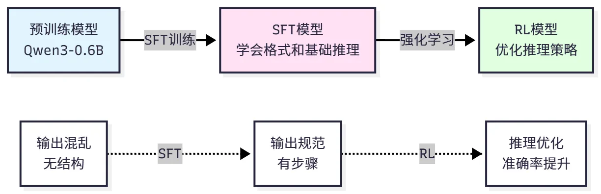
Figure 11.6 Role of SFT in Training Pipeline
11.3.2 LoRA: Parameter-Efficient Fine-Tuning
Directly fine-tuning the entire model requires substantial computational resources and memory. For Qwen3-0.6B (0.6B parameters), full fine-tuning requires about 12GB memory (FP16) or 24GB memory (FP32). For larger models (such as 7B, 13B), full fine-tuning is almost impossible on consumer-grade GPUs.
LoRA (Low-Rank Adaptation)<sup>[3]</sup> is a parameter-efficient fine-tuning method that only trains a small number of additional parameters while keeping the original model parameters frozen. The core idea of LoRA is: parameter changes during model fine-tuning can be represented by low-rank matrices.
Assume the original model's weight matrix is $W \in \mathbb{R}^{d \times k}$, and the fine-tuned weight is $W' = W + \Delta W$. LoRA assumes $\Delta W$ can be decomposed into the product of two low-rank matrices:
$$ \Delta W = BA $$
Where $B \in \mathbb{R}^{d \times r}$, $A \in \mathbb{R}^{r \times k}$, $r \ll \min(d, k)$ is the rank.
During forward propagation, the output is:
$$ h = Wx + \Delta Wx = Wx + BAx $$
The original model parameters $W$ remain frozen, only training $B$ and $A$.
Parameter count comparison: original model parameter count is $d \times k$, LoRA parameter count is $d \times r + r \times k = r(d + k)$. When $r \ll \min(d, k)$, LoRA parameter count is much smaller than the original model. For example, for $d=4096, k=4096, r=8$, original model parameter count is $4096 \times 4096 = 16,777,216$, LoRA parameter count is $8 \times (4096 + 4096) = 65,536$, a 256-fold reduction in parameters!
Therefore, we can summarize LoRA's advantages: significantly reduced memory usage, faster training speed, easy deployment, and prevention of overfitting. However, training effectiveness is usually somewhat worse than full parameter tuning.
As shown in Table 11.5, comparison of LoRA effects at different model scales.
Table 11.5 LoRA vs Full Fine-Tuning Comparison

LoRA's key hyperparameters include: rank (r), controlling the rank of LoRA matrices, larger means stronger expressiveness but more parameters, typical values 4-64, default 8; Alpha ($\alpha$), LoRA scaling factor, actual update is $\Delta W = \frac{\alpha}{r} BA$, controls LoRA's influence strength, typical value equals rank; target_modules, specifying which layers to apply LoRA, usually choosing attention layers (q_proj, k_proj, v_proj, o_proj), can also include MLP layers (gate_proj, up_proj, down_proj).
11.3.3 SFT Training Practice
Now let's conduct SFT training using HelloAgents. The complete training process includes: preparing dataset, configuring LoRA, setting training parameters, starting training, and saving model.
Basic training example:
from hello_agents.tools import RLTrainingTool

# Create training tool
rl_tool = RLTrainingTool()

# SFT training
result = rl_tool.run({
    # Training configuration
    "action": "train",
    "algorithm": "sft",

    # Model configuration
    "model_name": "Qwen/Qwen3-0.6B",
    "output_dir": "./models/sft_model",

    # Data configuration
    "max_samples": 100,     # Use 100 samples for quick test

    # Training parameters
    "num_epochs": 3,        # Train for 3 epochs
    "batch_size": 4,        # Batch size
    "learning_rate": 5e-5,  # Learning rate

    # LoRA configuration
    "use_lora": True,       # Use LoRA
    "lora_rank": 8,         # LoRA rank
    "lora_alpha": 16,       # LoRA alpha
})

print(f"\n✓ Training completed!")
print(f"  - Model save path: {result['model_path']}")
print(f"  - Training samples: {result['num_samples']}")
print(f"  - Training epochs: {result['num_epochs']}")
print(f"  - Final loss: {result['final_loss']:.4f}")
If the loss gradually decreases during training, it indicates the model is learning.
(1) Training Parameter Details
Let's understand the meaning and tuning suggestions for each training parameter in detail.
Data Parameters:
max_samples: Number of training samples to use. For quick testing, use 100-1000 samples; for complete training, recommend using all data (7473 samples). More data usually brings better results, but training time is also longer.split: Dataset split, default "train". Can be set to "train[:1000]" to use only the first 1000 samples.
Training Parameters:
num_epochs: Number of training epochs. 1 epoch means traversing the entire dataset once. Too few (1-2 epochs) may underfit, too many (>10 epochs) may overfit. Recommend starting from 3 epochs, observe loss curve and adjust.batch_size: Number of samples used per update. Larger is more stable but uses more memory. Recommend adjusting based on memory: 4GB memory use batch_size=1-2, 8GB memory use batch_size=4-8, 16GB memory use batch_size=8-16.learning_rate: Learning rate, controls parameter update step size. Too small (1e-6) converges slowly, too large (1e-3) may not converge. SFT recommends 5e-5, LoRA can be slightly larger (1e-4).
LoRA Parameters:
use_lora: Whether to use LoRA. Recommend always enabling unless there is sufficient memory.lora_rank: LoRA rank, controls expressiveness. 4-8 suitable for small tasks, 16-32 suitable for complex tasks, 64 suitable for large-scale fine-tuning.lora_alpha: LoRA scaling factor, usually set to 2 times the rank. When rank=8, alpha=16; when rank=16, alpha=32.
Optimizer Parameters:
optimizer: Optimizer type, default "adamw". AdamW is the most commonly used choice, can also try "sgd" or "adafactor".weight_decay: Weight decay, prevents overfitting. Default 0.01, can try 0.001-0.1.warmup_ratio: Learning rate warmup ratio. Learning rate increases linearly for the first warmup_ratio steps, then decays linearly. Default 0.1 (warmup for first 10% steps).
(2) Complete Training Example
Let's conduct a complete SFT training using all data and best practices:
from hello_agents.tools import RLTrainingTool

rl_tool = RLTrainingTool()

# Complete SFT training
result = rl_tool.run({
    "action": "train",
    "algorithm": "sft",

    # Model configuration
    "model_name": "Qwen/Qwen3-0.6B",
    "output_dir": "./models/sft_full",

    # Data configuration
    "max_samples": None,    # Use all data (7473 samples)

    # Training parameters
    "num_epochs": 3,
    "batch_size": 8,
    "learning_rate": 5e-5,
    "warmup_ratio": 0.1,
    "weight_decay": 0.01,

    # LoRA configuration
    "use_lora": True,
    "lora_rank": 16,        # Use larger rank
    "lora_alpha": 32,
    "lora_target_modules": ["q_proj", "k_proj", "v_proj", "o_proj"],

    # Other configurations
    "save_steps": 500,      # Save every 500 steps
    "logging_steps": 100,   # Log every 100 steps
    "eval_steps": 500,      # Evaluate every 500 steps
})

print(f"Training completed! Model saved at: {result['model_path']}")
This configuration is suitable for training on GPUs with 8GB memory, estimated to take 30-60 minutes.
(3) Training Monitoring and Debugging
During training, we need to monitor three key metrics. Loss should gradually decrease; if it doesn't decrease, learning rate may be too small or data may have problems; if it decreases then rises, learning rate may be too large or overfitting may occur. Gradient Norm should be in a reasonable range of 0.1-10; too large (>100) indicates gradient explosion and requires reducing learning rate; too small (<0.01) indicates gradient vanishing and requires checking model configuration. Learning Rate should change according to warmup strategy, linearly increasing for the first 10% steps, then linearly decaying to 0.
Common problems during training and solutions: when out of memory, reduce batch_size or max_length, use gradient accumulation or smaller model; when training is slow, increase batch_size, reduce logging frequency, or use mixed precision training; when loss doesn't decrease, increase learning rate, check data format, or increase training epochs; when overfitting, increase weight_decay, reduce training epochs, or use more data.
11.3.4 Model Evaluation
After training is complete, we need to evaluate the model's effectiveness. Evaluation metrics include:
Accuracy: Proportion of completely correct answers, most direct metric, range 0-1, higher is better.
Average Reward: Average reward across all samples, comprehensively considering accuracy, length, steps and other factors, range depends on reward function design.
Reasoning Quality: Clarity and logic of reasoning process, requires manual evaluation or specialized evaluation models.
Using HelloAgents to evaluate models:
from hello_agents.tools import RLTrainingTool

rl_tool = RLTrainingTool()

# Evaluate SFT model
eval_result = rl_tool.run({
    "action": "evaluate",
    "model_path": "./models/sft_full",
    "max_samples": 100,     # Evaluate on 100 test samples
    "use_lora": True,
})

eval_data = json.loads(eval_result)
print(f"\nEvaluation results:")
print(f"  - Accuracy: {eval_data['accuracy']}")
print(f"  - Average reward: {eval_data['average_reward']}")
print(f"  - Test samples: {eval_data['num_samples']}")
For small models like Qwen3-0.6B, achieving 40-50% accuracy on GSM8K after SFT is normal. Through reinforcement learning, we can further improve to 60-70%.
To better understand SFT's effectiveness, we can compare models at different stages:
# Evaluate pretrained model (without SFT)
base_result = rl_tool.run({
    "action": "evaluate",
    "model_path": "Qwen/Qwen3-0.6B",
    "max_samples": 100,
    "use_lora": False,
})
base_data = json.loads(base_result)

# Evaluate SFT model
sft_result = rl_tool.run({
    "action": "evaluate",
    "model_path": "./models/sft_full",
    "max_samples": 100,
    "use_lora": True,
})
sft_data = json.loads(sft_result)

# Compare results
print("Model comparison:")
print(f"Pretrained model accuracy: {base_data['accuracy']}")
print(f"SFT model accuracy: {sft_data['accuracy']}")
In this section, we learned about SFT's importance (learning format, establishing baseline), LoRA principles (low-rank decomposition, parameter efficiency), SFT training practice (parameter configuration, training monitoring), and model evaluation (accuracy, comparative analysis).